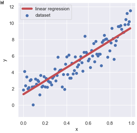
Polynomial regression is a technique to express a dataset with a linear regression model consisting of polynomial terms. Although we assume a linear relationship, we can reflect the non-linearity by including the non-linear effect in each polynomial term itself. Therefore, a polynomial-regression model can treat nonlinearity, so it sometimes becomes a powerful tool.
Especially, it’s a powerful technique, if you have an idea for a concrete expression of an expression.
In this post, we look at a process of polynomial-regression analyses with Python. The details of the theory are introduced in another post.
Import the Libraries
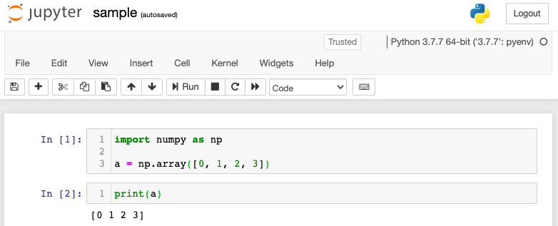
The code is written by Python. So firstly, we import the necessary library.
##-- For Numerical analyses
import numpy as np
##-- For Plot
import matplotlib.pylab as plt
import seaborn as sns
##-- For Linear Regression Analyses
from sklearn.linear_model import LinearRegression
Model Function
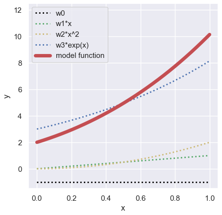
In this post, we adopt the following function as a polynomial regression model.
$$y =\omega_{0}+\omega_{1}x+\omega_{2}x^{2}+\omega_{3}e^{x},$$
where $\omega$ is the coefficient. Here, we assume $\omega$ as follows:
$$\begin{eqnarray*}
{\bf w^{T}}&&=\left(\omega_{0}\ \omega_{1}\ \omega_{2}\ \omega_{3}\right),\\
&&=\left(-1\ 1\ 2\ 3\right).
\end{eqnarray*}$$
Namely,
$$y =-1+x+2x^{2}+3e^{x}.$$
Create the Training Dataset
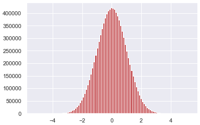
Next, we prepare the training dataset by adding the noise generated by “the Gaussian distribution”, which is also called “the Normal distribution”. With the noise function $\varepsilon(x)$, we can rewrite the model function as follows:
$$\begin{eqnarray*}
y =-1+x+2x^{2}+3e^{x} + \varepsilon(x),
\end{eqnarray*}$$
where $\varepsilon(x)$ is described as
$$\begin{eqnarray*}
\varepsilon(x)=\dfrac{1}{\sqrt{2\pi\sigma^{2}}}
e^{-\dfrac{(x-\mu)^{2}}{2\sigma^{2}}}.
\end{eqnarray*}$$
##-- Model Function
def func(param, X):
return param[0] + param[1]*X + param[2]*np.power(X, 2) + param[3]*np.exp(X)
x = np.arange(0, 1, 0.01)
param = [-1.0, 1.0, 2.0, 3.0]
np.random.seed(seed=99) # Set Random Seed
y_model = func(param, x)
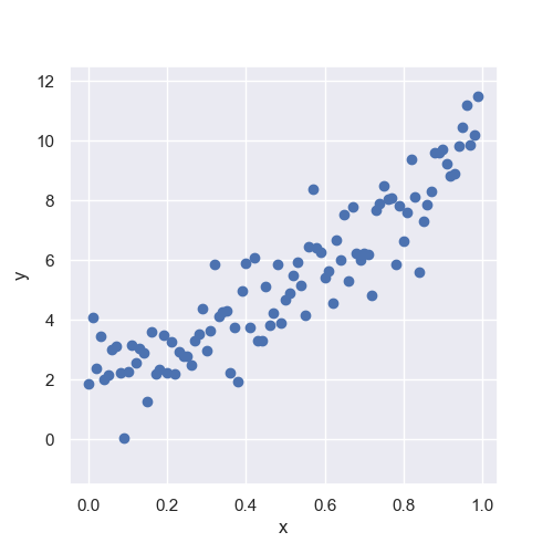
y_train = func(param, x) + np.random.normal(loc=0, scale=1.0, size=len(x))We can check the training dataset ($x$, $y_{\text{train}}$) as follows:
plt.figure(figsize=(5, 5), dpi=100)
sns.set()
plt.xlabel("x")
plt.ylabel("y")
plt.scatter(x, y_train, lw=1, color="b", label="toy dataset")
plt.plot(x, y_model, lw=5, color="r", label="model function")
plt.legend()
plt.show()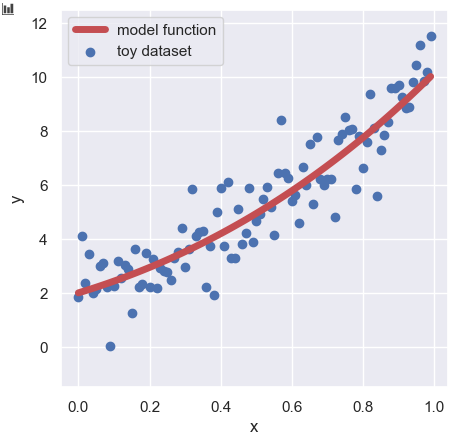
The details of the way to create the training dataset with the above model function are explained in another post.
Prepare the Dataset as Pandas DataFrame
Here, we prepare the dataset as Pandas DataFrame. First, we create empty DataFrame by “pd.DataFrame()“. Next, we create the values of each polynomial term in each column.
x_train = pd.DataFrame()

x_train["x"] = x
x_train["x^2"] = np.power(x, 2)
x_train["exp(x)"] = np.exp(x)
If you check only the first 5 lines of the created DataFrame, it will be as follows.
print( x_train.head() )

>>       x     x^2    exp(x)
>> 0  0.00  0.0000  1.000000
>> 1  0.01  0.0001  1.010050
>> 2  0.02  0.0004  1.020201
>> 3  0.03  0.0009  1.030455
>> 4  0.04  0.0016  1.040811
Note that since the constant term is treated as an intercept during the linear regression analysis, it is not necessary to create a column of constant terms (all values are “1”) here.
Polynomial Regression
Finally, we will perform linear regression analysis of polynomial terms from here!!
Then, we can apply a polynomial analysis to the above training dataset (x_train, y_train). Here, we use the “LinearRegression()” module from the scikit-learn library. And, create the instance “regressor” from “LinearRegression()”.
from sklearn.linear_model import LinearRegression
regressor = LinearRegression()
Then, we give the training dataset (x_train, y_train) to “regressor“, making “regressor” trained.
regressor.fit(x_train, y_train)Model training is over, so let’s predict.
y_pred = regressor.predict(x_train)Let’s see the prediction result.
plt.figure(figsize=(5, 5), dpi=100)
sns.set()
plt.xlabel("x")
plt.ylabel("y")
plt.scatter(x, y_train, lw=1, color="b", label="training dataset")
plt.plot(x, y_model, lw=3, color="r", label="model function")
plt.plot(x, y_pred, lw=3, color="g", label="Polynomial regression")
plt.legend()
plt.show()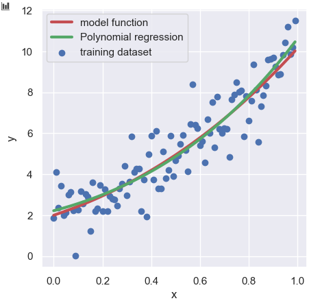
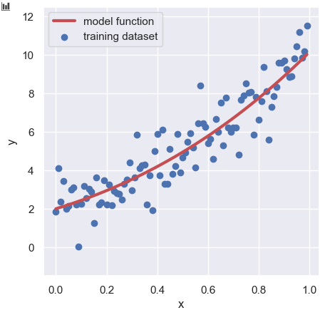
Above the plot, the red solid line, the green solid line, and the blue circles are described as the model function, the polynomial regression, and the training dataset, respectively. As you can see visually, the polynomial regression is in good agreement with the model function.
Coefficients of Polynomial Regression
Here, we have confirmed that the model function is reproduced well so far, let’s check the coefficients of the polynomial regression model.
We can confirm the intercept and coefficients by the methods “intercept_” and “coef_” against the regression instance “regressor”.
print("w0", regressor.intercept_, "\n", \
      "w1", regressor.coef_[0], "\n", \
      "w2", regressor.coef_[0], "\n", \
      "w3", regressor.coef_[0], "\n" )

>> w0 -5.385823038595163
>> w1 -4.479990435844182
>> w2 -0.187758224924017
>> w3  7.606988274352645
The estimated ${\bf w^{T}}$,
$$\begin{eqnarray*}
{\bf w^{T}}&&=\left(-5.4\ -4.5\ -0.2\ 7.6\right),
\end{eqnarray*}$$
deviates the one of the model function,
$$\begin{eqnarray*}
{\bf w^{T}}&&=\left(-1\ 1\ 2\ 3\right).
\end{eqnarray*}$$.
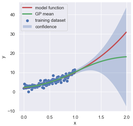
This deviation comes from the fact that the range of training data (0 to 1) is narrow. Therefore, if we increase the range of training data, the estimated value will close to the ones of the model function.
For example, when the range of training data is 0 to 2, ${\bf w^{T}}$ becomes $\left(-0.6\ 1.6\ 2.2\ 2.6\right)$. How is it? The estimation is very close to the correct answer.
Also, if the range of training data is 0 to 10, you can get the almost correct result.
Summary
We have briefly looked at the process of polynomial regression. Polynomial regression is a powerful and practical technique. However, without proper verification of the results, there is a risk of making a big mistake in predicting extrapolated values.
The author hopes this blog helps readers a little.