Linear regression analysis is one of the most basic data analyses. This method is based on the relationship between independent variables and dataset. Therefore, if the fit between the linear model and the dataset is well, an analysis with high model interpretability can be performed.
Purpose of this post
The purpose is to introduce the shortcode example for linear regression.
Explanation of Linear Regression
In this post, we just check the brief concept of linear regression. The details are introduced in another post. Please refer to it.
A representation of a linear regression is as follows:
$$y =\omega_{0}+\omega_{1}x_{1}+\omega_{2}x_{2}+…+\omega_{N}x_{N},$$
where $x_{i}$ is an independent variable and $\omega_{i}$ is a coefficient.
Here, for convenience, we adopt just one independent variable model. This is the most simple form everyone knows.
$$y =\omega_{0}+\omega_{1}x_{1}.$$
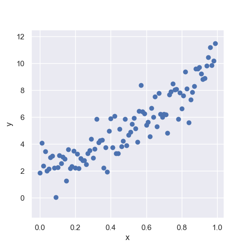
Training Dataset
We create the training dataset from the following code. How to create is introduced in another post.
import numpy as np
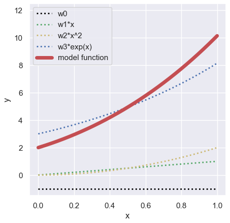
##-- Model Function for creating the toy dataset
def func(param, X):
return param[0] + param[1]*X + param[2]*np.power(X, 2) + param[3]*np.exp(X)
x = np.arange(0, 1, 0.01)
param = [-1.0, 1.0, 2.0, 3.0]
np.random.seed(seed=99) # Set Random Seed
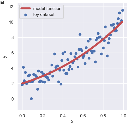
y_model = func(param, x)
y_train = func(param, x) + np.random.normal(loc=0, scale=1.0, size=len(x))Linear Regression Analyses
You can easily perform a linear regression analysis by the Scikit-learn module “LinearRegression()“. The procedure is as follows:
1. Create the instance of “LinearRegression()” as the name of “lr“
2. Train the model instance “lr” with the dataset by the “.fit()” module
3. Predict the training dataset by the “.predict()” module
from sklearn.linear_model import LinearRegression
lr = LinearRegression()
lr.fit(x.reshape(-1, 1), y_train)
y_pred = lr.predict(x.reshape(-1, 1))
Possibly, you have the question that what does “x.reshape(-1, 1)” mean. The answer is that we have to prepare input variables “x” as a two-dimensional array. You will see the following error message if you prepare “x” as a one-dimensional array.
ValueError: Expected 2D array, got 1D array instead:
” *************** Here depends on your code *************** “
Reshape your data either using array.reshape(-1, 1) if your data has a single feature or array.reshape(1, -1) if it contains a single sample.
In such a case, you have to convert “x” into a two-dimensional array by “x.reshape(-1, 1)“.
Congratulations!! Until here, the linear regression analysis is finished. You can confirm the result of your model as follows:
import matplotlib.pylab as plt
import seaborn as sns

plt.figure(figsize=(5, 5), dpi=100)
sns.set()
plt.xlabel("x")
plt.ylabel("y")
plt.ylim(-1.5, 12.5)
plt.scatter(x, y_train, lw=1, color="b", label="dataset")
plt.plot(x, y_pred, lw=5, color="r", label="linear regression")
plt.legend()
plt.show()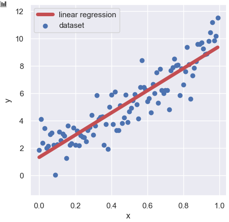
Summary
Contrary to the author’s intention, this blog has become a bit long. However, the important contents are as follows.
from sklearn.linear_model import LinearRegression
lr = LinearRegression()
lr.fit(x.reshape(-1, 1), y_train)
y_pred = lr.predict(x.reshape(-1, 1))
The point is that you can perform a linear regression analysis with JUST the 4 line code! The roles of each line are below.
1. Import the module
2. Create the model
3. Train the model with the dataset
4. Predict
I would be glad if you think a linear regression is easy!