We need a dataset to try out quickly something new method we learned. Therefore, it’s very important to get used to working with open datasets.
In this post, several open datasets, which are included in scikit-learn, will be introduced. From scikit-learn, we can easily and quickly use these datasets for regression and classification analyses.
The link to the code in the GitHub repository is here.
What is scikit-learn?
scikit-learn is one of the famous python libraries for machine learning. scikit-learn is easy to use, powerful, and including a variety of techniques. It can be widely used from statistical analysis to machine learning to deep learning.
Open Toy datasets in scikit-learn
scikit-learn is not only used to implement machine learning but also contains various datasets. it should be noted here that the toy dataset introduced below can be used offline once scikit-learn is installed.
The list of the datasets in scikit-learn is as follows. The reference is in the scikit-learn document.
- Boston house prices dataset (regression)
- Iris dataset (classification)
- Diabetes dataset (regression)
- Digits dataset (classification)
- Physical excercise linnerud dataset
- Wine dataset (classification)
- Breast cancer wisconsin dataset (classification)
By using scikit-learn, we can use the above datasets in the same way.
Let’s first take the Boston home price dataset as an example. Once you understand this example, you can treat the rest of the dataset as well.
Import common libraries
Here, import the commonly used python library.
Boston house prices dataset
This dataset is for regression analysis. Therefore, we can utilize this dataset to try a method for regression analysis you learned.
First, we import the dataset module from scikit-learn. The dataset is included in the sklearn.datasets module.
from sklearn.datasets import load_boston
Second, create the instance of the dataset. In this instance, various information is stored, i.e., the explanatory data, the names of features, the regression target data, and the description of the dataset. Then, we can extract and use information from this instance as needed.
# instance of the boston house-prices dataset
dataset = load_boston()
We can confirm the details of the dataset by the DESCR method.
print(dataset.DESCR)


>> .. _boston_dataset:
>>
>> Boston house prices dataset
>> ---------------------------
>>
>> **Data Set Characteristics:**
>>
>>     :Number of Instances: 506
>>
>>     :Number of Attributes: 13 numeric/categorical predictive. Median Value (attribute 14) is usually the target.
>>
>>     :Attribute Information (in order):
>>         - CRIM     per capita crime rate by town
>>         - ZN       proportion of residential land zoned for lots over 25,000 sq.ft.
>>         - INDUS    proportion of non-retail business acres per town
>>         - CHAS     Charles River dummy variable (= 1 if tract bounds river; 0 otherwise)
>>         - NOX      nitric oxides concentration (parts per 10 million)
>>         - RM       average number of rooms per dwelling
>>         - AGE      proportion of owner-occupied units built prior to 1940
>>         - DIS      weighted distances to five Boston employment centres
>>         - RAD      index of accessibility to radial highways
>>         - TAX      full-value property-tax rate per $10,000
>>         - PTRATIO  pupil-teacher ratio by town
>>         - B        1000(Bk - 0.63)^2 where Bk is the proportion of blacks by town
>>         - LSTAT    % lower status of the population
>>         - MEDV     Median value of owner-occupied homes in $1000's
>>
>>     :Missing Attribute Values: None
>>
>>     :Creator: Harrison, D. and Rubinfeld, D.L.
>>
>>     .
>>     .
>>     .
Next, we confirm the contents of the dataset.
The contents of the dataset variable “dataset” can be accessed by specific methods. In this variable, several kinds of information are stored. The list of them is as follows.
dataset.data: the explanatory-variable values
dataset.feature_names: the explanatory-variable names
dataset.target: values of the target variable
First, we take the data and the feature names of the explanatory variables.
# explanatory variables
X = dataset.data
# feature names
feature_names = dataset.feature_names
The data type of the above variable X is numpy array. For convenience, we convert the dataset into the Pandas DataFrame type. With the DataFrame type, we can easily manipulate the table-type dataset and perform the preprocessing.
# convert the data type from numpy array into pandas DataFrame
X = pd.DataFrame(X, columns=feature_names)
# display the first five rows.
print(X.head())


>>         CRIM    ZN  INDUS  CHAS    NOX  ...  RAD    TAX  PTRATIO       B  LSTAT
>>   0  0.00632  18.0   2.31   0.0  0.538  ...  1.0  296.0     15.3  396.90   4.98
>>   1  0.02731   0.0   7.07   0.0  0.469  ...  2.0  242.0     17.8  396.90   9.14
>>   2  0.02729   0.0   7.07   0.0  0.469  ...  2.0  242.0     17.8  392.83   4.03
>>   3  0.03237   0.0   2.18   0.0  0.458  ...  3.0  222.0     18.7  394.63   2.94
>>   4  0.06905   0.0   2.18   0.0  0.458  ...  3.0  222.0     18.7  396.90   5.33
Finally, we take the target-variable data.
# target variable
y = dataset.target
# display the first five elements.
print(y[0:5])


>>   [24.  21.6 34.7 33.4 36.2]
Now you have the explanatory variable X and the target variable y ready. In the real analysis, the process from here is performing preprocessing the data, creating the model, and validating the accuracy of the model.
You can do the same procedures for other datasets. The code for each dataset is described below.
Iris dataset
This dataset is for classification analysis.
from sklearn.datasets import load_iris


# instance of the iris dataset
dataset = load_iris()
# explanatory variables
X = dataset.data
# feature names
feature_names = dataset.feature_names
# convert the data type from numpy array into pandas DataFrame
X = pd.DataFrame(X, columns=feature_names)
# target variable
y = dataset.target
Diabetes dataset
This dataset is for regression analysis.
from sklearn.datasets import load_diabetes


# instance of the Diabetes dataset
dataset = load_diabetes()
# explanatory variables
X = dataset.data
# feature names
feature_names = dataset.feature_names
# convert the data type from numpy array into pandas DataFrame
X = pd.DataFrame(X, columns=feature_names)
# target variable
y = dataset.target
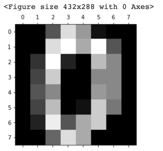
Digits dataset
This dataset is for classification analysis. It must be noted here that this dataset is image data. Therefore, the methods for taking each data are different from other datasets.
dataset.images: the raw image data
dataset.feature_names: the explanatory-variable names
dataset.target: values of the target variable
from sklearn.datasets import load_digits


# instance of the digits dataset
dataset = load_digits()
# explanatory variables
X = dataset.images  # X.shape is (1797, 8, 8)

# target variable(0, 1, 2, .., 8, 9)
y = dataset.target

# Display the image
import matplotlib.pyplot as plt
plt.gray()
plt.matshow(X[0])
plt.show()
Physical excercise linnerud dataset
This dataset is for multi-target regression analysis. In this dataset, the target variable has three outputs.
from sklearn.datasets import load_linnerud


# instance of the physical excercise linnerud dataset
dataset = load_linnerud()
# explanatory variables
X = dataset.data
# feature names
feature_names = dataset.feature_names
# convert the data type from numpy array into pandas DataFrame
X = pd.DataFrame(X, columns=feature_names)
# target variable
y = dataset.target

X.head()
print(y)
Wine dataset
This dataset is for classification analysis.
from sklearn.datasets import load_wine


# instance of the wine dataset
dataset = load_wine()
# explanatory variables
X = dataset.data
# feature names
feature_names = dataset.feature_names
# convert the data type from numpy array into pandas DataFrame
X = pd.DataFrame(X, columns=feature_names)
# target variable
y = dataset.target
Breast cancer wisconsin dataset
This dataset is for regression analysis.
from sklearn.datasets import load_breast_cancer


# instance of the Breast cancer wisconsin dataset
dataset = load_breast_cancer()
# explanatory variables
X = dataset.data
# feature names
feature_names = dataset.feature_names
# convert the data type from numpy array into pandas DataFrame
X = pd.DataFrame(X, columns=feature_names)
# target variable
y = dataset.target
Summary
In this post, we have seen several famous datasets in scikit-learn. Open datasets are important to try out quickly something new method we learned.
Therefore, let’s get used to working with open datasets.