

A linear-regression technique is one of the basic analysis methods, so it may become the first attempt to investigate the relationship between independent variables and dataset.
In this post, we look through briefly the theory of linear regression. This article focuses on the concept of linear regression, so it will help the readers to understand with imagination.
Code implemented by Python
The implementation of the linear-regression model by Python is introduced by another post. This post is for just the brief theory with the simplified concept.
What is the linear regression?
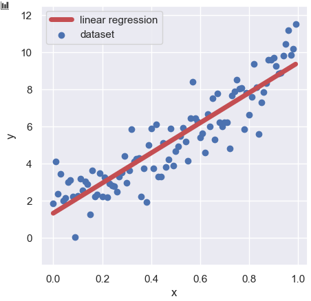
Linear regression is a technique to investigate the relationship between independent variables and a dataset. However, we assume that this relationship is linear. The most typical function would be:
$$y=ax+b,$$
Brief theory of linear regression
A representation of a linear regression is as follows:
$$y =\omega_{0}+\omega_{1}x_{1}+\omega_{2}x_{2}+…+\omega_{N}x_{N},$$
where $x_{i}$ is an independent variable and $\omega_{i}$ is a coefficient.
Besides, setting $x_{i}$ as $x_{1}=x$, $x_{2}=x^{2}$, and $x_{3}=e^{x}$, we can treat polynomial regression as the linear regression form:
$$y =\omega_{0}+\omega_{1}x+\omega_{2}x^{2}+\omega_{3}e^{x}.$$
The next step is to vectorize the above equation.
$$y=\left(\omega_{0}\ \omega_{1}\ \ldots\ \omega_{D}\right)\left(\begin{array}{ccc}1\\x_{1}\\\vdots\\x_{D}\\\end{array}\right).$$
$$\therefore y={\bf w^{T}}{\bf x},$$
where ${\bf w^{T}}$ is a coefficient vector and ${\bf x}$ is an independent variable vector. For the N dataset,
$$\left(\begin{array}{ccc}y_{1}\\y_{2}\\\vdots\\y_{N}\\\end{array}\right)=\left(\begin{array}{ccc}{\bf w^{T}}{\bf x_{1}}\\{\bf w^{T}}{\bf x_{2}}\\\vdots\\{\bf w^{T}}{\bf x_{N}}\\\end{array}\right).$$
As the matrix form, we can rewrite the above equation as follows:
$$\left(\begin{array}{ccc}y_{1}\\y_{2}\\\vdots\\y_{N}\\\end{array}\right)=\left(\begin{array}{ccccc}1&x_{11} &x_{12}&\ldots&x_{1D} \\1&x_{21} &x_{22}&\ldots&x_{2D}\\\vdots&&&&\vdots\\1&x_{N1} &x_{N2}&\ldots&x_{ND}\\\end{array}\right)\left(\begin{array}{ccc}\omega_{0}\\\omega_{1}\\\vdots\\\omega_{D}\\\end{array}\right).$$
$$\therefore{\bf y}\ ={\bf X}{\bf w}.$$
Our purpose is to estimate ${\bf w}$. Then, we will consider finding ${\bf w}$, which fits the dataset, namely minimizes the loss between the train data and the model-predicted data. We introduce the loss function of $E$ as follows:
$$\begin{eqnarray*}
E\left[ {\bf y}, {\bf \hat{y}}, {\bf X}; {\bf w} \right]\ &&=\sum^{n}_{n=1}\left(\hat{y}_{n} – y_{n} \right)^{2},\\ &&=\left({\bf \hat{y}} – {\bf X}{\bf w}\right)^{T}\left({\bf \hat{y}} – {\bf X}{\bf w}\right),
\end{eqnarray*}$$
where ${\bf \hat{y}}$ is the training data, and $E\left[ {\bf y}, {\bf \hat{y}}, {\bf X}; {\bf w} \right]$ is the loss between the train data(${\bf \hat{y}}$) and the model-predicted data(${\bf y}$). Note that this type of the loss function is called “Mean squared error”.
Here, we rewrite ${\bf w}$ as ${\bf w^{*}}$, which minimizes the loss $E\left[ {\bf y}, {\bf \hat{y}}, {\bf X}; {\bf w} \right]$, derived from the following relationship.
\begin{eqnarray*}
\dfrac{\partial E\left[ {\bf y}, {\bf \hat{y}}, {\bf X}; {\bf w} \right]}
{\partial {\bf w}} = 0
.
\end{eqnarray*}
From the above equation, we can obtain the solution ${\bf w^{*}}$ as follows:
\begin{eqnarray*}
\therefore
{\bf w^{*}}
=
\left(
{\bf X}^{T}{\bf X}
\right)^{-1}
{\bf X}^{T}
{\bf \hat{y}}
.
\end{eqnarray*}
Note that although the details of the derivation were skipped here, we can check the omitted process in the famous textbooks of machine learning or linear algebra.
The key is that all required information to estimate ${\bf w^{*}}$ is a training dataset(${\bf X}$ and ${\bf y}$). In addition, when we assume the form of the polynomial function, we can also judge the appropriateness of the assumed model.
Summary
We have briefly looked at the theory of linear regression. From the form of ${\bf w^{*}}=\left({\bf X}^{T}{\bf X}\right)^{-1}{\bf X}^{T}{\bf \hat{y}}$, you can understand that a linear regression analysis is on matric calculations.
In practice, there are few opportunities to be conscious of the calculation process. However, once you understand that linear regression is a matrix calculation, you can understand that the amount of calculation will become very large as the number of data increases.