Category: GPy

Gaussian Process is a powerful method to perform regression analyses. We can use it in regression analyses as the same as linear regression. However, Gaussian Process is based on the calculation of a probability distribution and it can be applied flexibly due to the Bayesian approach.

The main differences between Gaussian Process and linear regression are below.

1. Modeling with nonlinear
2. Model has information on both the estimation and the uncertainty.

The first one is that since this method can handle non-linearity, it is a highly expressive model. For example, linear regression analyses assumed the linear relationship between input variables and the output. Therefore, in principle, linear regression analysis is not suitable for datasets with non-linear relationships. In contrast, in such a dataset, we can apply the Gaussian Process regression.

The second one is that the output of the model has both information about the regression values and the confidence of the output. In other words, the Gaussian model tells us the confidence of results. This is completely different from linear regression.

Let’s see these differences concretely with a simple example. The complete notebook can be found on GitHub.

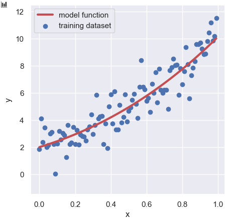
Create Training Dataset

Here, we create the training dataset. The way is to add the noise to the base function.

$$y =-1+x+2x^{2}+3e^{x} + \varepsilon(x).$$

$\varepsilon(x)$ is the noise function and described as follows:

$$\begin{eqnarray*}
\varepsilon(x)=\frac{1}{\sqrt{2\pi\sigma^{2}}}
e^{-\dfrac{(x-\mu)^{2}}{2\sigma^{2}}},
\end{eqnarray*}$$

where $\mu$ is the mean and $\sigma$ the standard deviation.

The code is below. The derails are introduced in another post.

import numpy as np
##-- Model Function for creating the train dataset
def func(param, X):
    return param[0] + param[1]*X + param[2]*np.power(X, 2) + param[3]*np.exp(X)

##-- Set Random Seed
np.random.seed(seed=99)

x = np.arange(0, 1, 0.01)
param = [-1.0, 1.0, 2.0, 3.0]

y_model = func(param, x)
y_train = func(param, x) + np.random.normal(loc=0, scale=1.0, size=len(x))

Gaussian Process Regression

In this analysis, we use “GPy“, the Gaussian Process library in Python. In this post, the version of GPy is assumed for “ver. 1.9.9”.

import GPy
print(GPy.__version__)

>> 1.9.9

Define “the kernel function”

First, we define the kernel function. There are many kinds of kernel functions. Here, we adopt “Matern52” as a kernel function. The theory of kernel functions is so deep, so beginners should use the representative one for a first try.

kernel = GPy.kern.Matern52(input_dim=1)

The option “input_dim” is the number of input variables. In this case, the input variable is just one “x”, so “input_dim = 1”.

Define the Model

Second, we define the Gaussian Process model as follows:

model = GPy.models.GPRegression(x.reshape(-1, 1), y_train.reshape(-1, 1), kernel=kernel)

There are three arguments, the input variable (x, y) and the kernel function.

Note that the dimensions of the input variable(x, y) must be two-dimensional. This is where beginners get stuck in debugging. We can easily confirm the dimensions as follows:

x_train.ndim  # x_train.ndim

>> 1

Whereas,

x_train.reshape(-1, 1).ndim  # y_train.reshape(-1, 1).ndim

>> 2

Optimize the Model

Now that we have defined the model, we can optimize it.

model.optimize()

GPy includes matplotlib inside, so you can quickly see the optimized model in just one line. Note that this method can be used when the number of the input variables is one. In multi variables case, the ability to plot in multiple dimensions is not supported.

model.plot(figsize=(5, 5), dpi=100, xlabel="x", ylabel="y")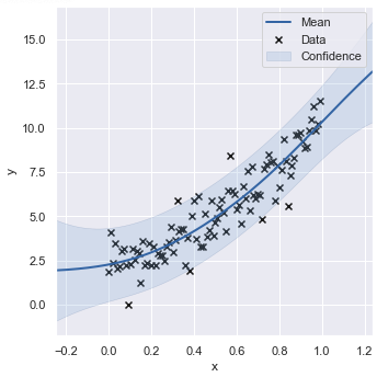

Prediction

Now that the model has been optimized, let’s check the predicted values and the confidence(uncertainty) with data outside the training data range. If all goes well, you’ll see a wider confidence interval in the data range outside the training data range.

Since the training data was in the range of 0 to 1, we will prepare the test data in the range of 0 to 2.

x_test = np.arange(0, 2, 0.01)

Then, predict the test data by the “.predict()” method.

y_mean, y_std = model.predict(x_test.reshape(-1, 1))

Note that there are two returned values from “model.predict()”. The first one is the regression value and the second one is the confidence interval. Here, it’s okay to think of the confidence interval as the standard deviation in the Gaussian function.

Finally, let’s plot the result.

import matplotlib.pylab as plt
import seaborn as sns

plt.figure(figsize=(5, 5), dpi=100)
sns.set()
plt.xlabel("x")
plt.ylabel("y")
plt.scatter(x, y_train, lw=1, color="b", label="training dataset")
plt.plot(x_test, func(param, x_test), lw=3, color="r", label="model function")
plt.plot(x_test, y_mean, lw=3, color="g", label="GP mean")
plt.fill_between(x_test, (y_mean + y_std).reshape(y_mean.shape[0]), (y_mean - y_std).reshape(y_mean.shape[0]), facecolor="b", alpha=0.3, label="confidence")
plt.legend(loc="upper left")
plt.show()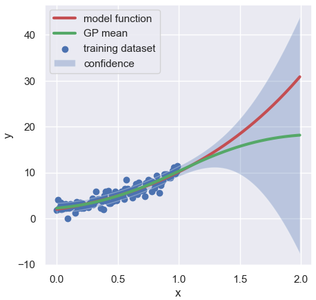

Congratulations!! It can be confirmed that as the range of the test data deviates from the training data, the predicted value also deviates and the confidence interval becomes wider.

Summary

From here, we have seen the process of Gaussian process regression with a simple example. Certainly, Gaussian process regression has the impression that it is difficult to attract attention as an analysis method because of its mathematical complexity. However, Gaussian process regression has information on confidence, making it possible to judge the validity of prediction.

The author would be happy if this post helps the reader to try Gaussian process analyses.