Category: NumPy

The toy dataset is useful when we attempt something new analysis method quickly, especially in regression analyses. In this post, we briefly see how to create a toy dataset with NumPy.

Then, let’s get started.

Import the Libraries

The code is written by Python. So firstly, we import the necessary library.

##-- For Numerical analyses
import numpy as np
##-- For Plot
import matplotlib.pylab as plt
import seaborn as sns

Define the Model Function

Here, we adopt the following function as an example.

$$y =-1+x+2x^{2}+3e^{x}.$$

The Python code for the above function is below.

def func(param, X):
    return param[0] + param[1]*X + param[2]*np.power(X, 2) + param[3]*np.exp(X)

For convenience, let’s create continuous data of x in the range 0 to 1 and check the behavior of the function.

x = np.arange(0, 1, 0.01)
param = [-1.0, 1.0, 2.0, 3.0]

y = func(param, x)

The behavior of (x, y) is as follows. The model function “y” is denoted by the red solid line. Note that, for visual clarity, the four polynomial terms, which construct the function, are added by the dashed line.

plt.figure(figsize=(5, 5), dpi=100)
sns.set()
plt.xlabel("x")
plt.ylabel("y")
plt.ylim(-1.5, 12.5)
plt.plot(x, y, lw=5, color="r", label="model function")
plt.legend()
plt.show()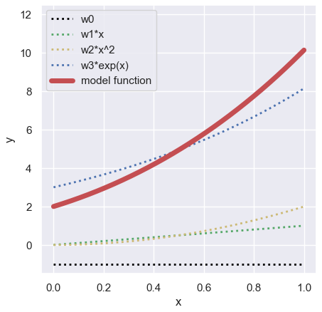

Generate the Noise

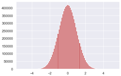
Next, we prepare the toy dataset by adding the noise into the above function. The noise is generated by “the Gaussian distribution”, which is also called “the Normal distribution”. In this case, the noise function $\varepsilon(x)$ can be written as follows:

$$\begin{eqnarray*}
\varepsilon(x)=\frac{1}{\sqrt{2\pi\sigma^{2}}}
e^{-\dfrac{(x-\mu)^{2}}{2\sigma^{2}}},
\end{eqnarray*}$$

where $\mu$ is the mean and $\sigma$ the standard deviation.

We can easily use this noise function $\varepsilon(x)$ by the NumPy module “np.random.normal()“.

noise = np.random.normal(
                            loc   = 0,
                            scale = 1,
                            size  = 10000000,
                        )
plt.hist(noise, bins=100, color="r")

“loc“, “scale“, and “size“, the arguments of “np.random.normal()“, are the mean($\mu$), the standard deviation($\sigma$), and the size of the output. As seen in the graph below, we can confirm the Gaussian distribution.

The Model Function with Noise

The code for the function with the noise is as follows:

$$y =-1+x+2x^{2}+3e^{x} + \varepsilon(x).$$

##-- Set Random Seed
np.random.seed(seed=99)

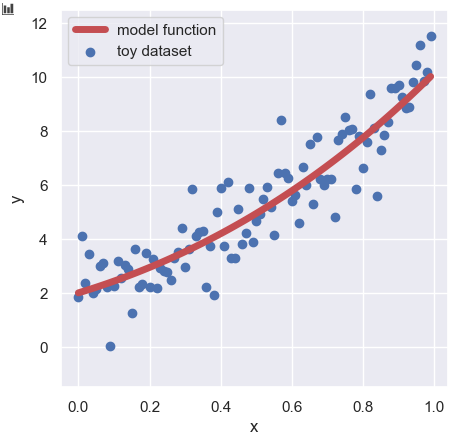
y_toy = func(param, x) + np.random.normal(loc=0, scale=1.0, size=len(x))

Finally, you can get the toy dataset $(x, y_toy)$!!
You can confirm the behavior of the toy dataset as follows:

plt.figure(figsize=(5, 5), dpi=100)
sns.set()
plt.xlabel("x")
plt.ylabel("y")
plt.ylim(-1.5, 12.5)
plt.scatter(x, y_toy, lw=1, color="b", label="toy dataset")
plt.plot(x, y, lw=5, color="r", label="model function")
plt.legend()
plt.show()