PyCaret is a powerful tool to compare models between different machine learning methods. The biggest feature of this library is the low code library for machine learning in Python. PyCaret is a wrapper including the famous machine learning libraries, scikit-learn, LightGBM, Catboost, XGBoost, and more.
To create one model, you may write an amount of code. So, you can imagine how difficult it is to compare models between different methods. However, PyCaret makes it easy to compare models, making it possible to experiment efficiently.
In this post, we will see the tutorial of PyCaret with a regression analysis against the Boston house prices dataset. The author will explain with the step-by-step guide in mind!!
The complete notebook can be found on GitHub.
Library version
PyCaret is now highly developed, so you should check the version of the library.
pycaret == 2.2.2
pandas == 1.0.5
scikit-learn == 0.23.2
matplotlib == 3.2.2
PyCaret can be easily installed by pip command as follows:
$pip install pycaretIf you want to define the version of PyCaret, you can use the following command.
$pip install pycaret==2.2.2Import Library
To start, we import the following libraries.
##-- PyCaret
import pycaret
from pycaret.regression import *
##-- Pandas
import pandas as pd
from pandas import Series, DataFrame
##-- Scikit-learn
import sklearn
Dataset
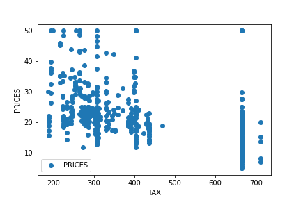
In this article, we use “Boston house prices dataset” from scikit-learn library, pubished by the Carnegie Mellon University. This dataset is one of the famous open-source datasets for testing new models.
From scikit-learn library, you can easily load the dataset. For convenience, we convert the dataset into the pandas-dataframe type, fundamental data structures in pandas.
from sklearn.datasets import load_boston
dataset = load_boston()

df = pd.DataFrame(dataset.data)
df.columns = dataset.feature_names
df["PRICES"] = dataset.target
df.head()

>>     CRIM     ZN    INDUS  CHAS  NOX    RM     AGE   DIS     RAD  TAX    PTRATIO  B       LSTAT  PRICES
>>  0  0.00632  18.0  2.31   0.0   0.538  6.575  65.2  4.0900  1.0  296.0  15.3     396.90  4.98   24.0
>>  1  0.02731   0.0  7.07   0.0   0.469  6.421  78.9  4.9671  2.0  242.0  17.8     396.90  9.14   21.6
>>  2  0.02729   0.0  7.07   0.0   0.469  7.185  61.1  4.9671  2.0  242.0  17.8     392.83  4.03   34.7
>>  3  0.03237   0.0  2.18   0.0   0.458  6.998  45.8  6.0622  3.0  222.0  18.7     394.63  2.94   33.4
>>  4  0.06905   0.0  2.18   0.0   0.458  7.147  54.2  6.0622  3.0  222.0  18.7     396.90  5.33   36.2
The details of the Boston house prices dataset are introduced in another post.
Before train the model, devide the dataset into train- and test- datasets. This is because we have to confirm whether the trained model has an ability to predict an unknown dataset. Here, we split the dataset into train and test datasets, as 8:2.
split_rate = 0.8
data = df.iloc[ : int(split_rate*len(df)), :]
data_pre = df.iloc[ int(split_rate*len(df)) :, :]
Set up the environment for PyCaret by the “setup()” function
Here, we set up the environment of the model by the “setup()” function. Arguments of the setup function are the input data, the name of the target data, and the “session_id”. The “session_id” equals to a random seed.
model_reg = setup(data = data, target = "PRICES", session_id=99)

>>             Data Type
>>     CRIM      Numeric
>>       ZN      Numeric
>>    INDUS      Numeric
>>     CHAS  Categorical
>>      NOX      Numeric
>>       RM      Numeric
>>      AGE      Numeric
>>      DIS      Numeric
>>      RAD      Numeric
>>      TAX      Numeric
>>  PTRATIO      Numeric
>>        B      Numeric
>>    LSTAT      Numeric
>>   PRICES        Label
Conveniently, PyCaret will predict the data type for each column as above. “Numeric” indicates the data is continuous values. On the other hand, “Categorical” means the data is NOT continuous values, for example, the season(spring, summer, fall, winter).
This is a very convenient function for quick data analysis!
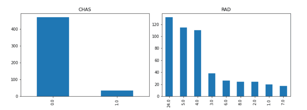
We have seen “CHAS” is NOT “Numeric”, where categorical data is NOT suitable for regression analysis. Then, we should drop the “CHAS” column from the dataset, and reset up the environment by the “setup()” function.
Note that, actually, “RAD” is also NOT continuous values. We can know this fact from the explanatory data analysis. You can check the details from the above link of another post, “Brief EDA for Boston House Prices Dataset“.
data = data.drop('CHAS', 1) # "1" indicate the columns.
model_reg = setup(data = data, target = "PRICES", session_id=99)

>>             Data Type
>>     CRIM      Numeric
>>       ZN      Numeric
>>    INDUS      Numeric
>>      NOX      Numeric
>>       RM      Numeric
>>      AGE      Numeric
>>      DIS      Numeric
>>      RAD      Numeric
>>      TAX      Numeric
>>  PTRATIO      Numeric
>>        B      Numeric
>>    LSTAT      Numeric
>>   PRICES        Label
Comparison Between All Models
PyCaret makes it possible to compare models easily with just one command as follows. We can compare the models by the evaluation metrics. Due to the smaller evaluation metrics(MAE, MSE, RMSE..), it turns out that superior solutions are based on decision tree-based methods.
compare_models()In this case, “CatBoost Regressor” is the best model. So, let’s construct the CatBoost-Regressor model. We use the “create_model” function and the argument of “catboost”. Another argument of “fold” is the number of cross-validation. In this case, we adopt “fold = 4”, then there are 4 (0~3) calculated results of each metric.
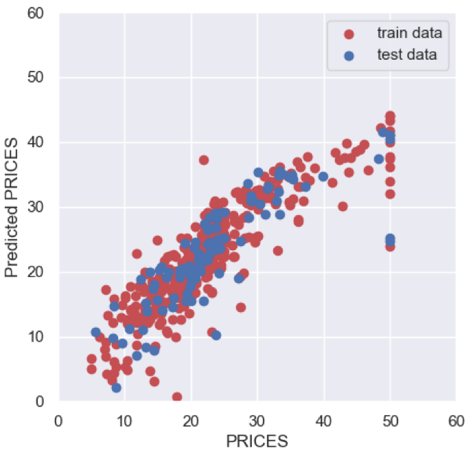
catboost = create_model("catboost", fold=4)Optimize Hyperparameter by Tune Model Module
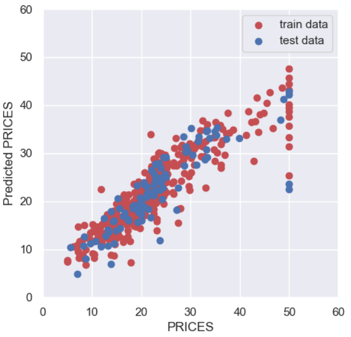
A tune-model module optimizes the created model by tuning the hyperparameters. You pass the created model to the tune-model function, “tune_model()”. An optimization is performed by a random grid search. After tuning, we can clearly see the improvement of MAE, 2.0685 to 1.9311.
tuned_model = tune_model(catboost)Visualization
It is also possible to visualize results by PyCaret. First, we check the contributions of the features by the “interpret_model()” module. The vertical axis indicates the explanatory features. And, the horizontal axis indicates the SHAP, contributions of the features into output. Each circle shows the value for every sample. From this figure, we can clearly see RM and LSTA are the key features to predict house prices.
interpret_model(tuned_model)Summary
We have seen the basic usage of PyCaret. Actually, PyCaret has various other functions, but the author has the impression that the functions are frequently renewed due to the high development speed.
The author’s recommended usage is to first check if there is a significant difference in accuracy between decision tree analysis and linear regression analysis. In general, decision tree-based methods tend to be more accurate than linear regression analysis. However, if you can expect some accuracy in the linear regression model, it is a good idea to try to understand the dataset from the linear regression analysis as the next step. This is because the model interpretability is higher in the linear regression analysis.
The essence of data science requires a deep understanding of datasets. To do so, it is important to repeat small trials quickly. PyCaret makes it possible to do such a thing more efficiently.
The author hopes this blog helps readers a little.