Regular expressions are one of the most essential skills, increasing your productivity. This article introduces how to use the “re” module, a famous build-in python library for regular expressions. It would be worth reading if you are unfamiliar with regular expressions.
This article is a long story, but informative. We can learn an example to use machine learning for finance. The topic is pair trading. We use machine learning to select the pair for long and short positions.
[News] A streamlit tutorial book has been published on Amazon Kindle!
I have published the book for a tutorial of Streamlit; “Tutorial of a Deployment of a Web app by Python and Streamlit for a Data Scientist”.
This new book is registered on Kindle Unlimited, so any member can read it !!
Features of this book
For beginners of Streamlit
Be aware of simple explanations
All with sample code
Introducing data analysis as a web application as an example
By streamlit, we can deploy our python script on a web app easier.
This post will see how to deploy our principal-component-analysis(PCA) code on a web app. In a web app format, we can try it in interactive. The origin of the PCA analysis in this post is introduced in another post.
It is easy to install streamlit by pip, just like any other Python module.
pip install streamlit
Run the web app
The web app will be opened by the following command in the web browser.
$ streamlit run main.py
Appendix: Dockerfile
If you use docker, you can use the Dockerfile described below. You can try the code in this post immediately.
FROM python:3.9

WORKDIR /opt
RUN pip install --upgrade pip
RUN pip install numpy==1.21.0 \
				pandas==1.3.0 \
				scikit-learn==0.24.2 \
				plotly==5.1.0 \
				matplotlib==3.4.2 \
				seaborn==0.11.1 \
				streamlit==0.84.1

WORKDIR /work
You can build a docker container from the docker image created from the Dockerfile.
Execute the following commands.
$ docker run -it -p 8888:8888 -v ~/(your work directory):/work <Image ID> bash
$ streamlit run main.py --server.port 8888
Note that “-p 8888: 8888” is an instruction to connect the host(your local PC) with the docker container. The first and second 8888 indicate the host’s and the container’s port numbers, respectively.
Besides, by the command “streamlit run ” with the option “–server.port 8888”, we can access a web app from a web browser with the URL “localhost: 8888”.
Please refer to the details on how to execute your python and streamlit script in a docker container in the following post.
import streamlit as st
import numpy as np
import pandas as pd
from sklearn.preprocessing import StandardScaler
from sklearn.metrics import accuracy_score
from sklearn.datasets import load_wine
from sklearn.decomposition import PCA
import plotly.graph_objects as go
Title
You can create the title quickly by ‘st.title()’.
‘st.title()’: creates a title box
# Title
st.title('PCA applied to Wine dataset')
Load and Show the dataset
First, we load the dataset by ‘load_wine()’, and set it as pandas DataFrame by ‘pd.DataFame’.
Second, we assign the columns of the dataset and the target variable. The columns of the dataset are stored in ‘dataset.feature_names’. Similarly, the target variable is also stored in ‘dataset.target’.
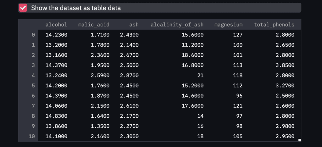
Third, we show the dataset as a table-data format if we check the checkbox. The checkbox is create by ‘st.checkbox()’, and a table data is shown by ‘st.dataframe()’.
‘st.checkbox()’: creates a check box, which returns True when checked. ‘st.dataframe()’: display the data frame of the argument.
# load wine dataset
dataset = load_wine()
# Prepare explanatory variable as DataFrame in pandas
df = pd.DataFrame(dataset.data)
# Assign the names of explanatory variables
df.columns = dataset.feature_names
# Add the target variable(house prices),
# where its column name is set "target".
df["target"] = dataset.target

# Show the table data when checkbox is ON.
if st.checkbox('Show the dataset as table data'):
    st.dataframe(df)
NOTE: Markdown
Here, it should be noted about ‘Markdown’, since, in the following descriptions, we will use the markdown format.
The markdown style is useful! For example, the following comment outed statement is shown in the web app as follows. With the markdown style, we can easily display the statement.
"""
# Markdown 1
## Markdown 2
### Markdown 3
"""
Standardization
Before performing the PCA, we have to perform standardization against explanatory variables.
# Prepare the explanatory and target variables
x = df.drop(columns=['target'])
y = df['target']

# Standardization
scaler = StandardScaler()
x_std = scaler.fit_transform(x)
You can refer to the details of standardization in the following post.
In this section, we perform the PCA and deploy it on streamlit.
We will create a design that interactively selects the number of principal components to be considered in the analysis. And, we select the principal components to be a plot.
Note that, we create these designs in the sidebar. It is easy by ‘st.sidebar’.
Number of principal components
First, we will create a design that interactively selects the number of principal components to be considered in the analysis.
By “st.sidebar”, the panels are created in sidebars.
And,
‘st.number_input()’: creates a panel, where we select the number.
# Number of principal components
st.sidebar.markdown(
r"""
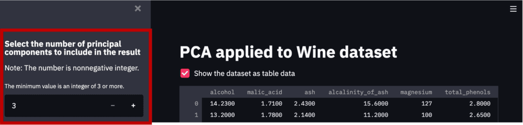
### Select the number of principal components to include in the result
Note: The number is nonnegative integer.
"""
)
num_pca = st.sidebar.number_input(
'The minimum value is an integer of 3 or more.',
value=3, # default value
step=1,
min_value=3)
Note that the part created by the above code is the red frame part in the figure below.
Perform the PCA
It is easy to perform the PCA by the “sklearn.decomposition.PCA()” module in scikit-learn. We pass the number of the principal components to the argument of “n_components”.
We create the panels in the sidebar to select the principal-component index to plot. This panel in the sidebar can be created by “st.sidebar.selectbox()”.
Note that we create the description as markdown in the sidebar using “st.sidebar”.
st.sidebar.markdown(
r"""
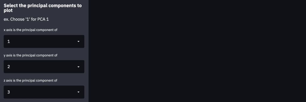
### Select the principal components to plot
ex. Choose '1' for PCA 1
"""
)
# Index of PCA, e.g. 1 for PCA 1, 2 for PCA 2, etc..
idx_x_pca = st.sidebar.selectbox("x axis is the principal component of ", np.arange(1, num_pca+1), 0)
idx_y_pca = st.sidebar.selectbox("y axis is the principal component of ", np.arange(1, num_pca+1), 1)
idx_z_pca = st.sidebar.selectbox("z axis is the principal component of ", np.arange(1, num_pca+1), 2)
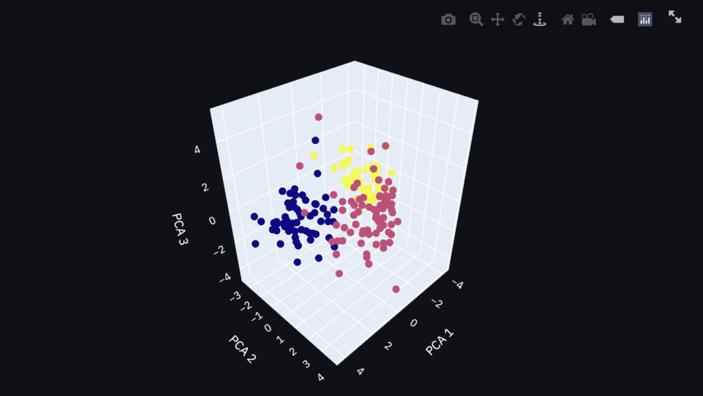
3D Plot by Plotly
Finally, let’s visualize the PCA result as a 3D plot. We can confirm the result interactively, e.g., zoom and scroll!
First, we prepare the label of each axis and the data to plot. We have already selected the principal-component index to plot.
Second, we visualize the result as a 3D plot by plotly. To visualize the result on the dashboard on Streamlit, we use the ‘st.plotly_chart()’ module, where the first argument is the graph instance created by plotly.
# Create an object for 3d scatter
trace1 = go.Scatter3d(
    x=x_plot, y=y_plot, z=z_plot,
    mode='markers',
    marker=dict(
        size=5,
        color=y,
        # colorscale='Viridis'
        )
)
# Create an object for graph layout
fig = go.Figure(data=[trace1])
fig.update_layout(scene = dict(
                    xaxis_title = x_lbl,
                    yaxis_title = y_lbl,
                    zaxis_title = z_lbl),
                    width=700,
                    margin=dict(r=20, b=10, l=10, t=10),
                    )
"""### 3d plot of the PCA result by plotly"""
# Plot on the dashboard on streamlit
st.plotly_chart(fig, use_container_width=True)
Since the graph is created as an HTML file, we can confirm it interactively.
Summary
In this post, we have seen how to deploy the PCA to a web app. I hope you experienced how easy it is to implement.
The author hopes you take advantage of Streamlit.
News: The Book has been published
The new book for a tutorial of Streamlit has been published on Amazon Kindle, which is registered in Kindle Unlimited. Any member can read it.
Visualizing the dataset is very important to understand a dataset.
However, the larger the number of explanatory variables, the more difficult it is to visualize that reflects the characteristics of the dataset. In the case of classification problems, it would be ideal to be able to classify a dataset with a small number of variables.
Principal Components Analysis(PCA) is one of the practical methods to visualize a high-dimensional dataset. This is because PCA is a technique to reduce the dimension of a dataset, i.e. aggregation of information of a dataset.
In this post, we will see how PCA can help you aggregate information and visualize the dataset. We use the wine classification dataset, one of the famous open datasets. We can easily use this dataset because it is already included in scikit-learn.
In the previous blog, exploratory data analysis(EDA) against the wine classification dataset is introduced. Therefore, you can check the detail of this dataset.
import numpy as np
import pandas as pd
from sklearn.preprocessing import StandardScaler
from sklearn.metrics import accuracy_score
from sklearn.datasets import load_wine
from sklearn.decomposition import PCA
import plotly.graph_objects as go
Load the dataset
dataset = load_wine()
Confirm the content of the dataset
The contents of the dataset are stored in the variable “dataset”. In this variable, several kinds of information are stored, i.e., the target-variable name and values, the explanatory-variable names and values, and the description of the dataset. Then, we have to take each of them separately.
dataset.target_name: the class labels of the target variable dataset.target: values of the target variable (class label) dataset.feature_names: the explanatory-variable names dataset.data: the explanatory-variable values
We can take the class labels and those unique data in the target variable.
There are three classes in the target variables(‘class_0’ ‘class_1’ ‘class_2’). These classes correspond to [0 1 2].
In other words, the problem is classifying wine into three categories from the explanatory variables.
Prepare the dataset as DataFrame in pandas
For convenience, we convert the dataset into the Pandas DataFrame type. With the DataFrame type, we can easily manipulate the table-type dataset and perform the preprocessing.
Here, let’s put all the data together into one Pandas DataFrame “df”.
In this dataset, there are 13 kinds of explanatory variables. Therefore, to visualize the dataset, we have to reduce the dimension of the dataset by PCA.
Preapare the Explanatory variables and the Target variable
First, we prepare the explanatory variables and the target variable, separately.
"""Prepare the explanatory and target variables"""
x = df.drop(columns=['target'])
y = df['target']
Standardize the Variables
Before performing PCA, we should standardize the numerical variables because the scales of variables are different. We can perform it easily by scikit-learn as follows.
Here, let’s perform the PCA analysis. It is easy to perform it using scikit-learn.
"""PCA: principal component analysis"""
# from sklearn.decomposition import PCA

pca = PCA(n_components=3)
x_pca = pca.fit_transform(x_std)
PCA can be done in just two lines.
The first line creates an instance to execute PCA. The argument “n_components” represents the number of principal components held by the instance. If “n_components = 3”, the instance holds the first to third principal components.
The second line executes PCA as an explanatory variable with the instance set in the first line. The return value is the result of being converted to the main component, and in this case, it contains three components.
Just in case, let’s check the shape of the obtained “x_pca”. You can see that there are 3 components and 178 data numbers.
print(x_pca.shape)

>>  (178, 3)
Visualize the dataset
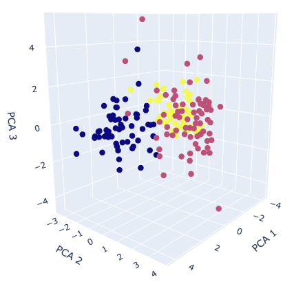
Finally, we visualize the dataset. We already obtained the 3 principal components, so it is a good choice to create the 3D scatter plot. To create the 3D scatter plot, we use plotly, one of the famous python libraries.
# import plotly.graph_objects as go

"""axis-label name"""
x_lbl, y_lbl, z_lbl = 'PCA 1', 'PCA 2', 'PCA 3'
"""data at eact axis to plot"""
x_plot, y_plot, z_plot = x_pca[:,0], x_pca[:,1], x_pca[:,2]

"""Create an object for 3d scatter"""
trace1 = go.Scatter3d(
    x=x_plot, y=y_plot, z=z_plot,
    mode='markers',
    marker=dict(
        size=5,
        color=y, # distinguish the class by color
        )
)
"""Create an object for graph layout"""
fig = go.Figure(data=[trace1])
fig.update_layout(scene = dict(
                    xaxis_title = x_lbl,
                    yaxis_title = y_lbl,
                    zaxis_title = z_lbl),
                    width=700,
                    margin=dict(r=20, b=10, l=10, t=10),
                    )
fig.show()
The colors correspond to the classification class. It can be seen from the graph that it is possible to roughly classify information-aggregated principal components.
If it is still difficult to classify after applying principal component analysis, the dataset may lack important features. Therefore, even if it is applied to the classification model, there is a high possibility that the accuracy will be insufficient. In this way, PCA helps us to consider the dataset by visualization.
Summary
We have seen how to perform PCA and visualize its results. One of the reasons to perform PCA is to consider the complexity of the dataset. When the PCA results are insufficient to classify, it is recommended to perform feature engineering.
The author hopes this blog helps readers a little.
Exploratory data analysis(EDA) is one of the most important processes in data analysis. To construct a machine-learning model adequately, understanding a dataset is important. Without appropriate EDA, there is no success. After the EDA, you will be able to effectively select models and perform feature engineering.
In this post, we use the wine classification dataset, one of the famous open datasets. We can easily use this dataset because it is already included in scikit-learn.
It’s very important to get used to working with open datasets. This is because, through an open dataset, we can quickly try out something new method we learned.
In the previous blog, the open dataset for regression analyses was introduced. This time, the author will introduce the open dataset that can be used for classification problems.
import numpy as np
import pandas as pd
from matplotlib import pyplot as plt
import seaborn as sns
from sklearn import preprocessing
from sklearn.model_selection import train_test_split
from sklearn.datasets import load_wine
dataset = load_wine()
Load the dataset
dataset = load_wine()
We can confirm the details of the dataset by the .DESCR method.
print(dataset.DESCR)


>> .. _wine_dataset:
>>
>> Wine recognition dataset
>> ------------------------
>>
>> **Data Set Characteristics:**
>>
>>     :Number of Instances: 178 (50 in each of three classes)
>>     :Number of Attributes: 13 numeric, predictive attributes and the class
>>     :Attribute Information:
>>  		- Alcohol
>>  		- Malic acid
>>  		- Ash
>> 		- Alcalinity of ash
>>  		- Magnesium>
>> 		- Total phenols
>>  		- Flavanoids
>>  		- Nonflavanoid phenols
>>  		- Proanthocyanins
>> 		- Color intensity
>>  		- Hue
>>  		- OD280/OD315 of diluted wines
>>  		- Proline
>>
>>      - class:
>>             - class_0
>>             - class_1
>>             - class_2
>>
>>     :Summary Statistics:
>>
>>     .
>>     .
>>     .
Confirm the content of the dataset
The contents of the dataset are stored in the variable “dataset”. In this variable, several kinds of information are stored, i.e., the target-variable name and values, the explanatory-variable names and values, and the description of the dataset. Then, we have to take each of them separately.
dataset.target_name: the class labels of the target variable dataset.target: values of the target variable (class label) dataset.feature_names: the explanatory-variable names dataset.data: the explanatory-variable values
We can take the class labels and those data in the target variable.
There are three classes in the target variables(‘class_0’ ‘class_1’ ‘class_2’). In other words, it can be understood that it is a problem of classifying wine into three categories from the explanatory variables.
You can see that the explanatory variables have multiple kinds. A description of each variable can be found in “dataset.DESCR”.
Convert the dataset into DataFrame in pandas
For convenience, we convert the dataset into the Pandas DataFrame type. With the DataFrame type, we can easily manipulate the table-type dataset and perform the preprocessing.
Here, let’s put all the data together into one Pandas DataFrame “df”.
Fortunately, there is no missing value! This fact is because this dataset is created carefully. Note that, however, there are usually many problems we have to deal with a real dataset.
Confirm the basic Descriptive Statistics values
We can calculate the basic descriptive statistics values with just 1 sentence!
Especially, it is worth to focus on “mean” and “std” as a first attention.
We can know the average from “mean” so that it makes it possible to judge a value is higher or lower. This feeling is important for a data scientist.
Next, “std” represents the standard deviation, which is an indicator of how much the data is scattered from “mean”. For example, “std” will be small if each value exists almost average.
It should be noted that the variance equals the square of the standard deviation, and the word “variance” may be more common for a data scientist. It is no exaggeration to say that the information in a dataset is contained in the variance. In other words, we cannot get any information if all values are the same. Therefore, it’s okay to delete the variable with zero variance.
Histogram Distribution
Data with variance is the data that is worth paying attention to. So let’s actually visualize the distribution of the data.
Seeing is believing!
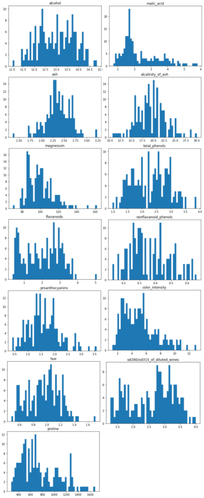
We can perform the histogram plotting by “plt.hist()” in “matplotlib”, a famous library for visualization. The argument “bins” can control the fineness of plot.
for name in f.columns:
    plt.title(name)
    plt.hist(f[name], bins=50)
    plt.show()
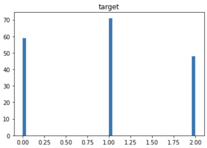
The distribution of the target variable is as follows. You can see that each category has almost the same amount of data. If the number of data is biased by category, you should pay attention to the decrease in accuracy due to imbalance.
The distributions of the explanatory variables are below. We can see the difference in variance between the explanatory variables.
Summary
We have seen how to perform EDA briefly. The purpose of EDA is to properly identify the nature of the dataset. Proper EDA can make it possible to explore the next step effectively, e.g. feature engineering and modeling methods.
In the case of classification problems, principal component analysis can be considered as a deeper analysis method. I will introduce it in another post.
This article introduces the three famous low-code python libraries for Machine learing, i.e., PyCaret, TPOT, and LazyPredict. It would be worth to read if you are interested in a low-code library for Machine learning.
A recursive function may be unfamiliar, especially to a beginner. This is because the concept is abstract, so that we don’t realize the opportunity to use it.
In this post, a brief description and an example of a recursive function are introduced. Through this example, the readers may realize it is helpful to keep your code simple.
What is a Recursive function?
A recursive function is a function that calls itself.
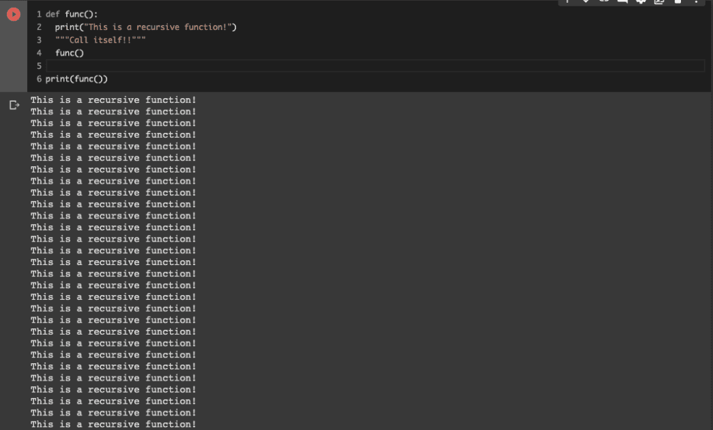
For example, the following code is the simple example.
It should be noted that, as a sensible reader may notice, running this function leads to an infinite loop.
def func():
  print("This is a recursive function!")
  """Call itself!!"""
  func()

print(func())
When to use it?
A function is a converter that performs one process. Therefore, a recursive function would be practical when creating a function that does the same thing multiple times.
Replacing similar processing with a recursive function leads to code simplification. Let’s experience it with the following simple example.
Example: factorial calculation
Here, one example is introduced. We will create the function for factorial calculations. Factorial calculations are like below.
$$N!=N\times(N-1)\times…\times2\times1$$
Without Recursive function
First, let’s implement without a recursive function. The code is below.
"""factorial calculation without recursive function"""
def factorial_nonrecursive(x):
  result = 1
  """N!=1*2*...*(N-1)*N"""
  for i in range(1, x+1):
    result = i*result
  return result


"""ex. 4! = 1*2*3*4 = 24"""
result = factorial_nonrecursive(4)
print(f"factorial: {result}")


>> factorial: 24
It may seem complicated at first glance, but the above code is just multiplying in order from 1 using for loop.
With Recursive function
Next, we perform refactoring of the above code with a recursive function. The code after refactoring is as follows.
"""factorial calculation with recursive function"""
def factorial_recursive(x):
  if x == 1:
    return 1
  else:
    return x*factorial_recursive(x-1)


"""ex. 4! = 1*2*3*4 = 24"""
result = factorial_recursive(4)
print(f"factorial: {result}")


>> factorial: 24
Did you realize that the code has become so simple?
Since the code is simple, it is easy to understand that the “factorial_recursive(x)” performs multiplication of the argument “x” with the previous returned result of this function.
Appendix: about Computational Cost
Here, we check the computational cost. We compare the calculating times between the above functions we created.
We import the necessary modules.
from time import time  # calculate time
import sys
sys.setrecursionlimit(50000) # Set the upper limit of the number of recursion
import numpy as np
from matplotlib import pyplot as plt
By the following codes, we get the time from begin to finish of calculating $N!$, where $N=10000$.
The first is the case with a recursive function.
N = 10000
cal_time_recursive = []
for i in range(1, N+1):
  begin_time = time()
  result = factorial_recursive(i)
  end_time = time()
  cal_time_recursive.append(end_time - begin_time)
The second is the case without a recursive function.
N = 10000
cal_time_nonrecursive = [] # calculation time
for i in range(1, N+1):
  begin_time = time()
  result = factorial_nonrecursive(i)
  end_time = time()
  cal_time_nonrecursive.append(end_time - begin_time)
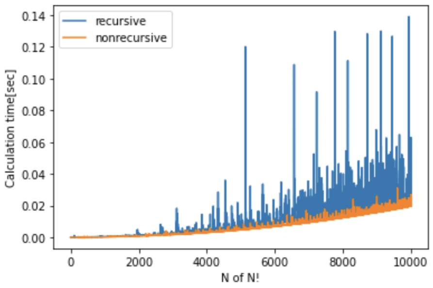
Finally, let’s check the graph of the calculation time of N! For N. The red and blue lines indicate the with-recursive and without-recursive cases, respectively.
You can see that the calculation time tends to be longer overall with recursion. This result would be due to the increase in the number of processes associated with the function calling itself sequentially. As you can see, recursive functions can simplify your code, but in some cases, they can take longer than usual.
Summary
A recursive function is a function that calls itself. Although it is unfamiliar with a python beginner, it is helpful to keep your code simple.
If you come across a situation where you can use it, please use it positively.
I have published the book for a tutorial of Streamlit; “Tutorial of a Deployment of a Web app by Python and Streamlit for a Data Scientist”.
This new book is registered on Kindle Unlimited, so any member can read it !!
Features of this book
For beginners of Streamlit
Be aware of simple explanations
All with sample code
Introducing data analysis as a web application as an example
What is Streamlit?
Streamlit is a wonderful library, making it easier and faster to build a web app for your data science project. By Streamlit, we can easily convert python script into a web app. Namely, we can publish our data analyses as a web app.
Articles about Streamlit have been posted in the past. The book was created with detailed explanations added. Especially, if you want to study all at once, please check it!
Most of data scientists may use CSV files instead of Excel format files(.xls or .xlsx). A CSV file is useful because of its simple format or rule(comma separated). However, you may encounter the situation that you want to use an Excel format file. This article tells how to treat an Excel format file step-by-step.
An example of data analyses in business fields using PyCaret. PyCaret is a low-code machine learning library, making it possible to build machine-learning models faster and compare them. Besides, in this article, there is a description of how to add custom a metric in PyCaret.