pd.melt() may be unfamiliar to a python beginner. It might be familiar for us to convert a long DataFrame into a wide DataFrame as preprocessing. Note that examples of a long DataFrame and a wide DataFrame are described in this article. We use the pd.melt() function when performing its inverse conversion, i.e., converting a wide DataFrame into a long DataFrame. I sometimes encounter to use this function when I analyze stock prices. You may have an opportunity to use it.
An article introducing a notable PyTorch-based library. PyTorch is a library for deep learning, however, Pytorch Tabular is a library for table data. In general, tree-based methods are popular for table data. Therefore, it is worth checking that the new library, based on the deep learing library, has appeared.
In sound analyses, we will encounter unfamiliar features such as spectrogram. We can learn what such features are in this article using librosa, a python library for sound analyses.
The machine learning approaches, such as decision-tree-based methods and linear regression, have been already introduced in other posts. These approaches are practical in real data science tasks.
However, deep learning approaches are also essential skills for a data scientist. In real, deep learning would be a more powerful approach when a dataset is larger than that of Boston house prices.
In this post, we will see a brief description of how to apply a neural network to the Boston house prices dataset.
from sklearn.datasets import load_boston
from sklearn import preprocessing
from sklearn.metrics import r2_score
import pandas as pd
import numpy as np
import matplotlib.pylab as plt
import seaborn as sns
sns.set()
import torch
import torch.nn as nn
import torch.nn.functional as F
import torch.optim as optim
Load the Dataset
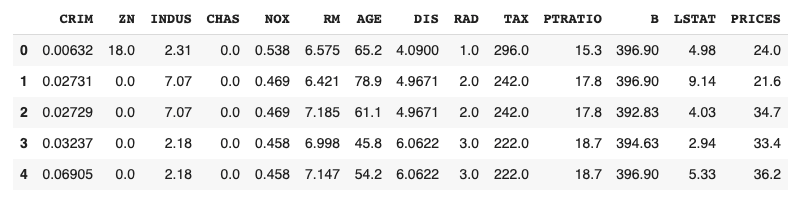
In this post, we use the Boston house prices dataset in the scikit-learn library. We can easily load the dataset by just two lines below.
# from sklearn.datasets import load_boston
dataset = load_boston()
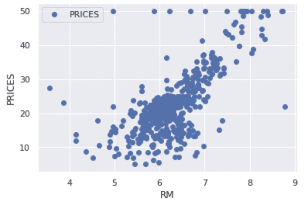
Let’s try to check the correlation between only “PRICES” and “RM”.
# import matplotlib.pylab as plt
f.plot(x="RM", y="PRICES", style="o")
plt.ylabel("PRICES")
plt.show()
Variables to be used
TargetName = "PRICES"
FeaturesName = [
              #-- "Crime occurrence rate per unit population by town"
              "CRIM",
              #-- "Percentage of 25000-squared-feet-area house"
              'ZN',
              #-- "Percentage of non-retail land area by town"
              'INDUS',
              #-- "Index for Charlse river: 0 is near, 1 is far"
              'CHAS',
              #-- "Nitrogen compound concentration"
              'NOX',
              #-- "Average number of rooms per residence"
              'RM',
              #-- "Percentage of buildings built before 1940"
              'AGE',
              #-- 'Weighted distance from five employment centers'
              "DIS",
              ##-- "Index for easy access to highway"
              'RAD',
              ##-- "Tax rate per $100,000"
              'TAX',
              ##-- "Percentage of students and teachers in each town"
              'PTRATIO',
              ##-- "1000(Bk - 0.63)^2, where Bk is the percentage of Black people"
              'B',
              ##-- "Percentage of low-class population"
              'LSTAT',
              ]
We prepare the input and target variables as “X” and “Y”.
X = f[FeaturesName]
Y = f[TargetName]
Standardize the Variables
We need to standardize or normalize the numerical variable in neural network analysis. This is because the magnitude of each variable affects its scale of parameters in a neural network. Therefore, the difference in the scale of the variables would make training of the model difficult.
From the above reason, we perform the standardization into the variables. In mathematically, the definition of the conversion of standardization is as follows.
To validate the performance of the trained model against unseen data, we have to split the dataset into the train data and the test data.
We pass the dataset “(X, Y)” to the “train_test_split()” function. The rate of the train data and the test data is defined by the argument “test_size”. Here, the rate is set to be “8:2”. And, “random_state” is set for reproducibility. You can use any number.
# from sklearn.model_selection import train_test_split
X_train, X_test, Y_train, Y_test = train_test_split(X_std, Y, test_size=0.2, random_state=99)
Define a Neural network model by PyTorch
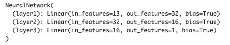
We define a neural network model. The model has three fully connected layers.
In “__init__()”, we define the layers we will use. For example, the first layer “self.layer1” has defined by “nn.Linear()” in PyTorch, where the input and output sizes are 13(X.shape[1]) and 32, respectively. Note that the input size 13 is automatically determined from the number of input variables in the dataset, whereas the output size is arbitrary and you have to decide. Similarly, in the second(third) layer, the input size has been automatically determined by the output size of the previous layer. In contrast, the output size is arbitrary and you have to decide. Namely, you can design the neural network structure by output sizes.
In “forward()”, we define the neural network structure. The input data is “x”. And, the “x” is passed into “self.layer1(x)”, where its output is given into the activation function “F.relu()”. Note that the output of the final(third) layer doesn’t have to be applied in the activation function. It is because the final-layer output is the predicted housing prices!
# import torch
# import torch.nn as nn
# import torch.nn.functional as F

class NeuralNetwork(nn.Module):
        def __init__(self):
            super(NeuralNetwork, self).__init__()
            self.layer1 = nn.Linear(X.shape[1], 32) # input: X.shape[1]=13, output: 32
            self.layer2 = nn.Linear(32, 16)
            self.layer3 = nn.Linear(16, 1)

        def forward(self, x):
            x = F.relu( self.layer1(x) )
            x = F.relu( self.layer2(x) )
            x = self.layer3(x)

            return x

model = NeuralNetwork()
print(model)
Convert data into a Tensor
In PyTorch, we have to explicitly convert the NumPy array(or pandas DataFrame) into a tensor. The conversion can be performed by “torch.tensor()”, where the param “type” is for specifying a data type.
It must be noted that the data shape of the prediction data will be (***, 1), whereas the data shape of “Y_train” is (***, ). These differences will cause the problem in calculating the loss in training. Therefore, we should reshape the data shape of “Y_train” before converting it into a tensor.
# Convert into tensor
x = torch.tensor(np.array(X_train), dtype=torch.float)
y = torch.tensor(np.array(Y_train).reshape(-1, 1), dtype=torch.float)
Define an Optimizer
We define an optimizer. PyTorch covers many optimization algorithms. The popular and basic ones are SGD and Adam.
Here, we choose the SGD algorithm as an optimizer.
# import torch.optim as optim
optimizer = optim.SGD(model.parameters(), lr=0.005)
We passed the two arguments “model.parameters()” and “lr=0.005”.
The first one is the parameters of the neural network model. The optimizer updates these parameters in each training cycle.
The second parameter is the learning rate. The learning rate is a parameter that indicates how much the model parameters are updated at once. Basically, gradually updating the parameters will surely lead to the optimum solution. On the other hand, it takes time to learn. Therefore, we need to think about the learning rate and find an appropriate value.
If you would like to use Adam as an optimizer, instead of the above codes, specify as follows.
We define a loss function. PyTorch covers many types of loss functions. Here, we use the mean squared error as a loss function.
# define loss function
loss_function = nn.MSELoss()
Train the Model
Finally, we can train the model !
At each epoch, we performs:
Initialize the gradient of the model parameters
Calculate the loss
Calculate the gradient of the model parameters by backpropagation
Update the model parameters
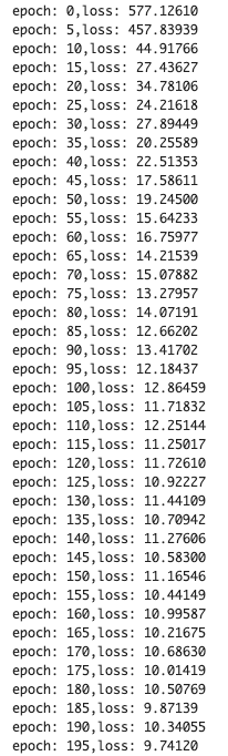
We set epochs as 200. Then, we repeat the above 200 times.
The loss would be gradually decreasing. It indicates that the training model is being well done !
# Epoch
epochs = 200

for i in range(epochs):
    # initialize the gradient of model parameters
    optimizer.zero_grad()

    # calculate the loss
    y_val = model(x)
    loss = loss_function(y_val, y)
    # Backpropagation
    loss.backward()
    # Update parameters
    optimizer.step()
    if (i % 5) == 0:
      print('epoch: {},'.format(i) + 'loss: {:.5f}'.format(loss))
Validation
To validate the performance of the model, we predict the training and validation data. It should be noted here that we have to convert the tensor into the NumPy array after prediction.
We calculate $R^{2}$ score to confirm the prediction accuracy.
$R^{2}$ is the index for how much the model is fitted to the dataset. When $R^{2}$ is close to $1$, the model accuracy is good. Conversely, when $R^{2}$ approaches $0$, it means that the model accuracy is poor.
We can calculate $R^{2}$ by the “r2_score()” function in scikit-learn.
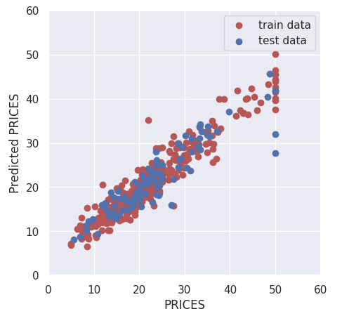
We have seen the Neural Network analysis constructed by PyTorch against the Boston house prices dataset. Although we use a very simple network structure, the accuracy of the validation data improved more than that of linear regression.
The author hopes this blog helps readers a little.
This article is so informative! We can learn how to utilize pycaret, a low-code python library for machine learning, in time series forecasting problems.
KNIME is an end-to-end data analysis platform that enables data linkage, integration, and analysis, which is developed as an open-source project. This article introduces how to use pycaret in KNIME.
This article treats several kinds of validation. Validation is so important in data analyses. It might be that validation is the first topic that a data science beginner should learn.
Low-code/Auto machine learning tools have been recently a hot topic, so it is worth to paid attention to. In this article, Pycaret and H2O Automl, one of the famous Low-code machine learning tools, are introduced.
Streamlit makes it easier and faster to make your python script a web app. This means we can publish our codes as a web app!
In this post, we will see how to deploy our linear-regression-analysis code on a web app. In a web app format, we can try it in interactive. The origin of the linear regression analysis in this post is introduced in another post.
If the docker is available, you can use the Dockerfile in the following post, making it easy to prepare an environment for streamlit. Then, you can try the code in this post immediately.
The web app will be opened by the following command in the web browser.
$ streamlit run Boston_House_Prices.py
Import libraries
import streamlit as st
import numpy as np
import pandas as pd
import matplotlib.pyplot as plt
import seaborn as sns
sns.set()
from sklearn.datasets import load_boston
from sklearn import preprocessing
from sklearn.model_selection import train_test_split
from sklearn.linear_model import LinearRegression
from sklearn.metrics import r2_score
Title
You can create the title quickly by ‘st.title()’.
‘st.title()’: creates a title box
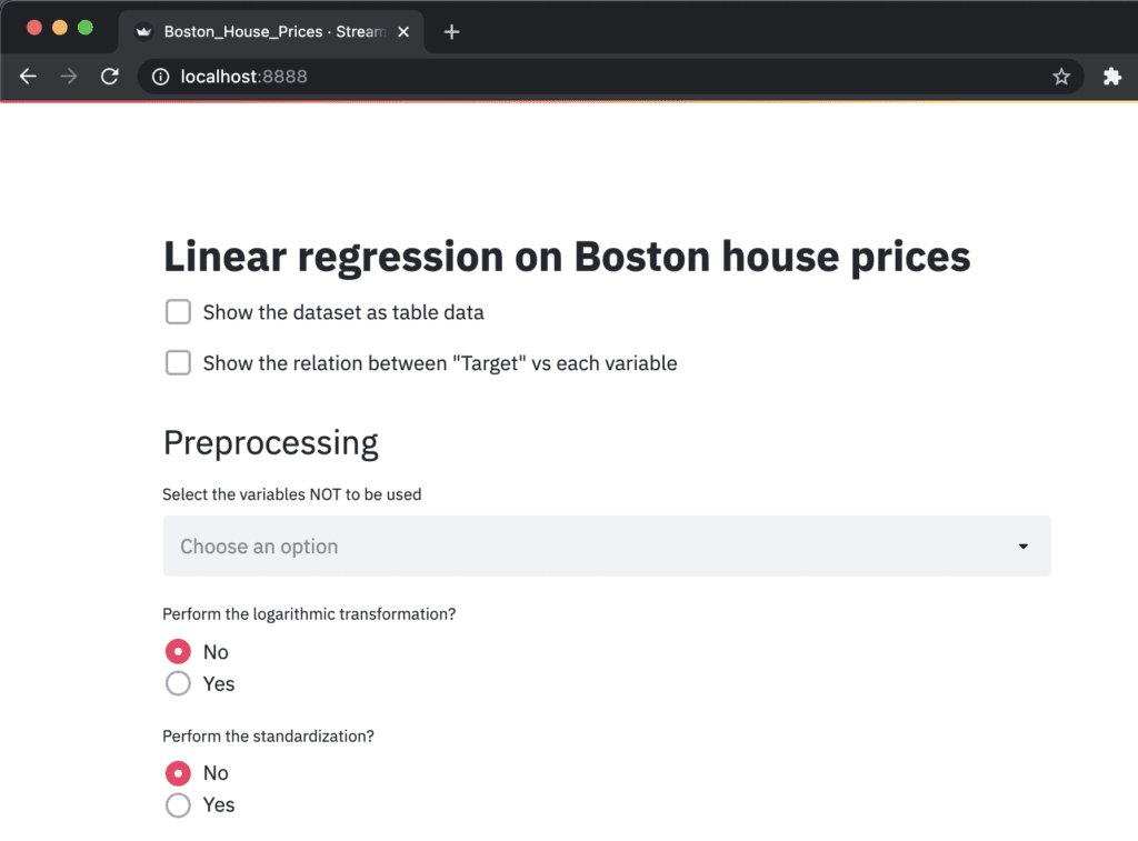
st.title('Linear regression on Boston house prices')
Load and Show the dataset
First, we load the dataset by ‘load_boston()’, and set it as pandas DataFrame by ‘pd.DataFame’.
Second, we assign the columns of the dataset and the target variable. The columns of the dataset are stored in ‘dataset.feature_names’. Similarly, the target variable is also stored in ‘dataset.target’.
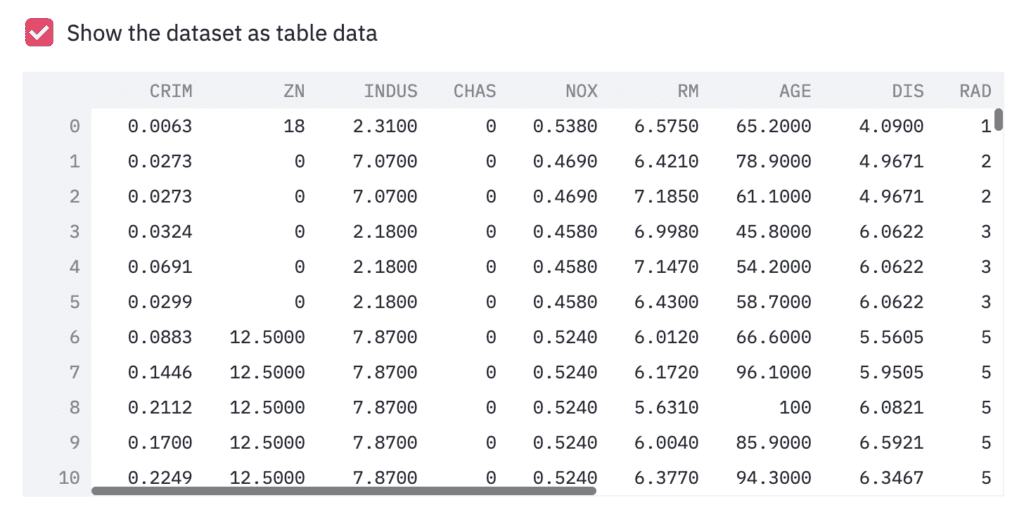
Third, we show the dataset as a table-data format, if we check the checkbox. The checkbox is create by ‘st.checkbox()’, and a table data is shown by ‘st.dataframe()’.
‘st.checkbox()’: creates a check box, which returns True when checked. ‘st.dataframe()’: display the data frame of the argument.
# Read the dataset
dataset = load_boston()
df = pd.DataFrame(dataset.data)
# Assign the columns into df
df.columns = dataset.feature_names
# Assign the target variable(house prices)
df["PRICES"] = dataset.target

# Show the table data
if st.checkbox('Show the dataset as table data'):
	st.dataframe(df)
For convenience, let’s create the box, where we can see a relationship between the target variable and the explanatory variables interactively.
‘st.checkbox()’: creates a check box, which returns True when checked. ‘st.selectbox()’: returns one element, we selected, from the argument.
# Check an exmple,  "Target" vs each variable
if st.checkbox('Show the relation between "Target" vs each variable'):
	checked_variable = st.selectbox(
		'Select one variable:',
		FeaturesName
		)
	# Plot
	fig, ax = plt.subplots(figsize=(5, 3))
	ax.scatter(x=df[checked_variable], y=df["PRICES"])
	plt.xlabel(checked_variable)
	plt.ylabel("PRICES")
	st.pyplot(fig)
Preprocessing
Here, we select the variables we will NOT use. We define the list ‘FeaturesName’, including the names of the explanatory variables.
# Explanatory variable
FeaturesName = [\
              #-- "Crime occurrence rate per unit population by town"
              "CRIM",\
              #-- "Percentage of 25000-squared-feet-area house"
              'ZN',\
              #-- "Percentage of non-retail land area by town"
              'INDUS',\
              #-- "Index for Charlse river: 0 is near, 1 is far"
              'CHAS',\
              #-- "Nitrogen compound concentration"
              'NOX',\
              #-- "Average number of rooms per residence"
              'RM',\
              #-- "Percentage of buildings built before 1940"
              'AGE',\
              #-- 'Weighted distance from five employment centers'
              "DIS",\
              ##-- "Index for easy access to highway"
              'RAD',\
              ##-- "Tax rate per $100,000"
              'TAX',\
              ##-- "Percentage of students and teachers in each town"
              'PTRATIO',\
              ##-- "1000(Bk - 0.63)^2, where Bk is the percentage of Black people"
              'B',\
              ##-- "Percentage of low-class population"
              'LSTAT',\
              ]
In streamlit, the multi-selection is available by ‘st.multiselect()’. We pass the variables for multi-selections to ‘st.multiselect()’.
‘st.multiselect()’: returns the multi elements, we selected, from the argument.
"""
## Preprocessing
"""
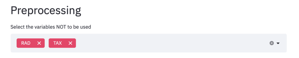
# Select the variables NOT to be used
Features_chosen = []
Features_NonUsed = st.multiselect(
'Select the variables NOT to be used',
FeaturesName)
Multiple selected variables are stored in ‘Features_NonUsed’, which will NOT be used. Let’s remove this unused variable from the dataset ‘df’.
df = df.drop(columns=Features_NonUsed)
NOTE: Markdown
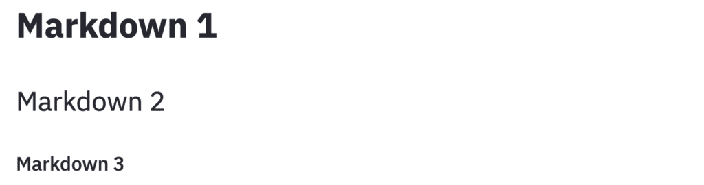
Here, it should be noted about ‘Markdown’. The markdown style is useful! For example, the following comment outed statement is shown in web app as follows. With the markdown style, we can easily display the statement.
"""
# Markdown 1
## Markdown 2
### Markdown 3
"""
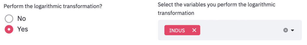
Next, as preprocessing, logarithmic conversion and standardization are performed. For logarithmic transformation, we select the variables that will be performed. On the other hand, for standardization, we take the form of selecting variables that won’t be performed.
The corresponding part of the code related to logarithmic conversion is as follows.
‘st.beta_columns(2)’: creates 2 columns ‘.radio()’: Put a box to select one from an argument.
left_column, right_column = st.beta_columns(2)
bool_log = left_column.radio(
			'Perform the logarithmic transformation?',
			('No','Yes')
			)

df_log, Log_Features = df.copy(), []
if bool_log == 'Yes':
	Log_Features = right_column.multiselect(
					'Select the variables you perform the logarithmic transformation',
					df.columns
					)
	# Perform logarithmic transformation
	df_log[Log_Features] = np.log(df_log[Log_Features])
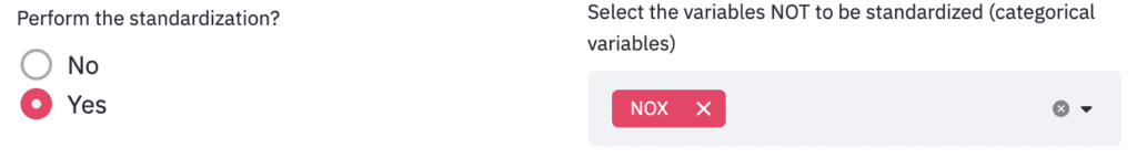
And, the corresponding part of the code related to standardization is as follows.
left_column, right_column = st.beta_columns(2)
bool_std = left_column.radio(
			'Perform the standardization?',
			('No','Yes')
			)

df_std = df_log.copy()
if bool_std == 'Yes':
	Std_Features_chosen = []
	Std_Features_NonUsed = right_column.multiselect(
					'Select the variables NOT to be standardized (categorical variables)',
					df_log.drop(columns=["PRICES"]).columns
					)
	for name in df_log.drop(columns=["PRICES"]).columns:
		if name in Std_Features_NonUsed:
			continue
		else:
			Std_Features_chosen.append(name)
	# Perform standardization
	sscaler = preprocessing.StandardScaler()
	sscaler.fit(df_std[Std_Features_chosen])
	df_std[Std_Features_chosen] = sscaler.transform(df_std[Std_Features_chosen])
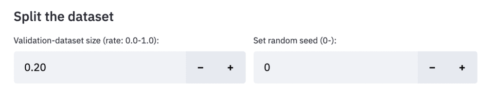
Split the dataset
To validate the model, we split the dataset into training and validation datasets. Interactively get information and split the dataset. Concretely, we put the boxes of the validation dataset size and the random seed.
Here, we use the following functions.
‘st.beta_columns(2)’: creates 2 columns ‘.number_input()’: Add a detail info to ‘st.beta_columns()’
Here, predict the training and validation data. Note that we have to perform logarithmic conversion against the variable we appointed.
Y_pred_train = regressor.predict(X_train)
Y_pred_val = regressor.predict(X_val)

# Inverse logarithmic transformation if necessary
if "PRICES" in Log_Features:
	Y_pred_train, Y_pred_val = np.exp(Y_pred_train), np.exp(Y_pred_val)
	Y_train, Y_val = np.exp(Y_train), np.exp(Y_val)
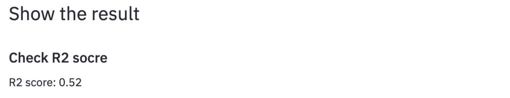
Here we use the R2 value as a validation indicator. Let’s calculate R2 of the validation dataset and display it in streamlit. You can easily do it with’st.write’.
"""
## Show the result
### Check R2 socre
"""
R2 = r2_score(Y_val, Y_pred_val)
st.write(f'R2 score: {R2:.2f}')
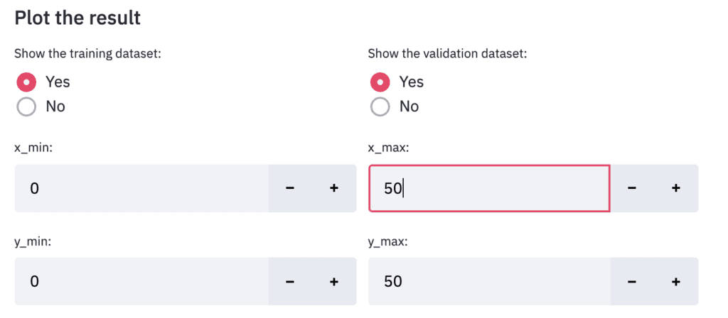
Plot
Finally, let’s output the result. Design the display settings for training data and verification data to be interactive. It is also designed to be able to interactively change the value range for the axes of the graph in the same way.
"""
### Plot the result
"""
left_column, right_column = st.beta_columns(2)
show_train = left_column.radio(
'Show the training dataset:',
('Yes','No')
)
show_val = right_column.radio(
'Show the validation dataset:',
('Yes','No')
)
# default axis range
y_max_train = max([max(Y_train), max(Y_pred_train)])
y_max_val = max([max(Y_val), max(Y_pred_val)])
y_max = int(max([y_max_train, y_max_val]))
# interactive axis range
left_column, right_column = st.beta_columns(2)
x_min = left_column.number_input('x_min:',value=0,step=1)
x_max = right_column.number_input('x_max:',value=y_max,step=1)
left_column, right_column = st.beta_columns(2)
y_min = left_column.number_input('y_min:',value=0,step=1)
y_max = right_column.number_input('y_max:',value=y_max,step=1)
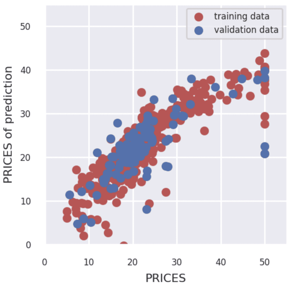
fig = plt.figure(figsize=(3, 3))
if show_train == 'Yes':
plt.scatter(Y_train, Y_pred_train,lw=0.1,color="r",label="training data")
if show_val == 'Yes':
plt.scatter(Y_val, Y_pred_val,lw=0.1,color="b",label="validation data")
plt.xlabel("PRICES",fontsize=8)
plt.ylabel("PRICES of prediction",fontsize=8)
plt.xlim(int(x_min), int(x_max)+5)
plt.ylim(int(y_min), int(y_max)+5)
plt.legend(fontsize=6)
plt.tick_params(labelsize=6)
st.pyplot(fig)
In this short post, we construct the environment for streamlit by docker. We create a docker image from a Dockerfile. And, we will see how to construct and run a docker container, and build a web app on its container.
Dockerfile
The entire contents of the Dockerfile are as follows.
FROM python:3.8.8

RUN pip install --upgrade pip
RUN pip install streamlit==0.78.0 \
				numpy==1.20.1 \
				pandas==1.2.3 \
				matplotlib==3.3.4 \
				seaborn==0.11.1 \
				scikit-learn==0.24.1

WORKDIR /work
We create the docker image based on the python image, whose version is 3.8.8.
And, we upgrade pip, to install the external python libraries. In addition to streamlit, to make things easier later, we also install numpy, pandas, matplotlib, seaborn, and scikit-learn.
Note that the last sentense ‘WORKDIR /work’ indicates that the current directory is set at ‘/work/’ after we enter the docker container.
Build a Dockerfile
Let’s create a docker image from the Dockerfile. Execute the following command in the directory where the Dockerfile exists.
$ docker build .
After building the docker image, you can confirm the result by the following command. Later, we will use the ‘IMAGE ID’.
$ docker images
Run a docker container
Here, we run the docker container from the above docker image. The command format is as follows.
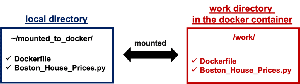
$ docker run -it -p 8888:8888 -v ~/mounted_to_docker/:/work <IMAGE ID> bash

'-p 8888:8888':
-> Allows the port, whose number is 8888, in a docker container

'-v ~/mounted_to_docker/:/work':
->Synchronizes the local directory you specified('~/mounted_to_docker/') with the directory in the container('/work').
$ docker run -it -p 8888:8888 -v ~/mounted_to_docker/:/work 8316e8947747 bash
When the docker container was successfully running, you would be in the container.
Your local directory ‘~/mounted_to_docker/’ is mounted to the working directory ‘/work’ in the container.
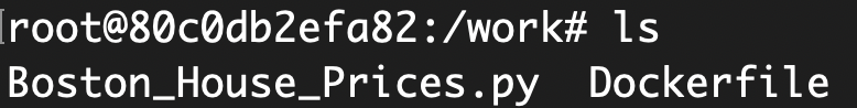
By the ‘ls’ command, you can check whether your local directory is mounted to the working directory in the container.
Run streamlit
In the container, it is possible to use streamlit. You can execute your python script designed with streamlit as follows.
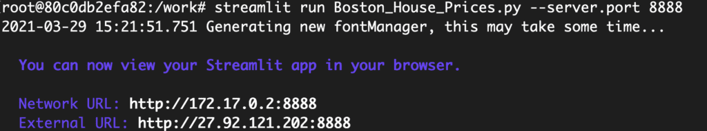
$ streamlit run Boston_House_Prices.py --server.port 8888
The ‘Network URL: http://172.17.0.2:8888’ is combined to ‘localhost:8888’. Therefore, you can view your web app created from ‘Boston_House_Prices.py’ at ‘localhost:8888’ in a web browser.
Congulaturation!! You have prepared the environment for using strea.
Announcement
The new book for a tutorial of Streamlit has been published on Amazon Kindle, which is registered in Kindle Unlimited. Any member can read it !
Streamlit is a fantastic library, making it easier and faster to make your python script a web app. This library makes it possible to publish your code as a web app! In addition, streamlit is designed with a simple UX, low code, and a readable official document.
In this post, we will see how to set up the environment of streamlit. In another post, we will deploy your data analysis on your web app, i.e., to publish your data analysis code as an interactive format.
Book was published
The new book for a tutorial of Streamlit has been published on Amazon Kindle, which is registered in Kindle Unlimited. Any member can read it !
The execute command is as follows. Your python script(sample.py) will be converted into a web app. A web app will open in a web browser.
$ streamlit run sample.py
Your app can be accessed from a web browser with “localhost:8888” of the URL.
Note that you can kill the web app by “control + C”(for Mac) or “Ctrl + C”(for Windows) in the terminal or the command prompt.
Once you run a python script, you can modify the script interactively. For example, after editing and saving the script, you can confirm the result by reloading the browser.
NOTE) Set up by Docker
If you use docker, it is easy to create an environment for streamlit. You can easily create it from Dockerfile.
FROM python:3.8.8

WORKDIR /opt
RUN pip install --upgrade pip
RUN pip install streamlit==0.78.0

WORKDIR /work
Build a docker image from a Dockerfile. Move the directory where the Dockerfile exists.
$ docker build .
Check the docker image created from Dockerfile by the following command.
$ docker images
Then, create the docker container from the docker image.
$ docker run -it -p 8888:8888 -v ~/(local folder PATH):/(container work directory PATH) <Image ID> bash

# ex.) docker run -it -p 8888:8888 -v ~/streamlit-demo:/work 109bbbac097f bash
You can execute streamlit as follows.
$ streamlit run sample.py --server.port 8888
From the above sequence, your app can be accessed by the URL “localhost:8888” in a web browser.