

Exploratory data analysis(EDA) is one of the most important processes in data analysis. To construct a machine-learning model adequately, understanding a dataset is important. Without appropriate EDA, there is no success. After the EDA, you will be able to effectively select models and perform feature engineering.
In this post, we use the wine classification dataset, one of the famous open datasets. We can easily use this dataset because it is already included in scikit-learn.
It’s very important to get used to working with open datasets. This is because, through an open dataset, we can quickly try out something new method we learned.
In the previous blog, the open dataset for regression analyses was introduced. This time, the author will introduce the open dataset that can be used for classification problems.
Import Library
import numpy as np
import pandas as pd
from matplotlib import pyplot as plt
import seaborn as sns
from sklearn import preprocessing
from sklearn.model_selection import train_test_split
from sklearn.datasets import load_wine
dataset = load_wine()
Load the dataset
dataset = load_wine()We can confirm the details of the dataset by the .DESCR method.
print(dataset.DESCR)


>> .. _wine_dataset:
>>
>> Wine recognition dataset
>> ------------------------
>>
>> **Data Set Characteristics:**
>>
>>     :Number of Instances: 178 (50 in each of three classes)
>>     :Number of Attributes: 13 numeric, predictive attributes and the class
>>     :Attribute Information:
>>  		- Alcohol
>>  		- Malic acid
>>  		- Ash
>> 		- Alcalinity of ash
>>  		- Magnesium>
>> 		- Total phenols
>>  		- Flavanoids
>>  		- Nonflavanoid phenols
>>  		- Proanthocyanins
>> 		- Color intensity
>>  		- Hue
>>  		- OD280/OD315 of diluted wines
>>  		- Proline
>>
>>      - class:
>>             - class_0
>>             - class_1
>>             - class_2
>>
>>     :Summary Statistics:
>>
>>     .
>>     .
>>     .
Confirm the content of the dataset
The contents of the dataset are stored in the variable “dataset”. In this variable, several kinds of information are stored, i.e., the target-variable name and values, the explanatory-variable names and values, and the description of the dataset. Then, we have to take each of them separately.
dataset.target_name: the class labels of the target variable
dataset.target: values of the target variable (class label)
dataset.feature_names: the explanatory-variable names
dataset.data: the explanatory-variable values
We can take the class labels and those data in the target variable.
"""target-variable name"""
print(dataset.target_names)
"""target-variable values"""
print(dataset.target)


>>  ['class_0' 'class_1' 'class_2']
>>  [0 0 0 0 0 0 0 0 0 0 0 0 0 0 0 0 0 0 0 0 0 0 0 0 0 0 0 0 0 0 0 0 0 0 0 0 0
>>   0 0 0 0 0 0 0 0 0 0 0 0 0 0 0 0 0 0 0 0 0 0 1 1 1 1 1 1 1 1 1 1 1 1 1 1 1
>>   1 1 1 1 1 1 1 1 1 1 1 1 1 1 1 1 1 1 1 1 1 1 1 1 1 1 1 1 1 1 1 1 1 1 1 1 1
>>   1 1 1 1 1 1 1 1 1 1 1 1 1 1 1 1 1 1 1 2 2 2 2 2 2 2 2 2 2 2 2 2 2 2 2 2 2
>>   2 2 2 2 2 2 2 2 2 2 2 2 2 2 2 2 2 2 2 2 2 2 2 2 2 2 2 2 2 2]
There are three classes in the target variables(‘class_0’ ‘class_1’ ‘class_2’). In other words, it can be understood that it is a problem of classifying wine into three categories from the explanatory variables.
Next, let’s take the explanatory variables.
"""explanatory-variable name"""
print(dataset.feature_names)
"""explanatory-variable values"""
print(dataset.data)


>>  ['alcohol', 'malic_acid', 'ash', 'alcalinity_of_ash', 'magnesium', 'total_phenols', 'flavanoids', 'nonflavanoid_phenols', 'proanthocyanins', 'color_intensity', 'hue', 'od280/od315_of_diluted_wines', 'proline']
>>  [[1.423e+01 1.710e+00 2.430e+00 ... 1.040e+00 3.920e+00 1.065e+03]
>>   [1.320e+01 1.780e+00 2.140e+00 ... 1.050e+00 3.400e+00 1.050e+03]
>>   [1.316e+01 2.360e+00 2.670e+00 ... 1.030e+00 3.170e+00 1.185e+03]
>>   ...
>>   [1.327e+01 4.280e+00 2.260e+00 ... 5.900e-01 1.560e+00 8.350e+02]
>>   [1.317e+01 2.590e+00 2.370e+00 ... 6.000e-01 1.620e+00 8.400e+02]
>>   [1.413e+01 4.100e+00 2.740e+00 ... 6.100e-01 1.600e+00 5.600e+02]]
You can see that the explanatory variables have multiple kinds. A description of each variable can be found in “dataset.DESCR”.
Convert the dataset into DataFrame in pandas
For convenience, we convert the dataset into the Pandas DataFrame type. With the DataFrame type, we can easily manipulate the table-type dataset and perform the preprocessing.
Here, let’s put all the data together into one Pandas DataFrame “df”.
(NOTE) df is an abbreviation for data frame.
"""Prepare explanatory variable as DataFrame in pandas"""
df = pd.DataFrame(dataset.data)
df.columns = dataset.feature_names
"""Add the target variable to df"""
df["target"] = dataset.target
print(df.head())


>>     alcohol  malic_acid   ash  ...  od280/od315_of_diluted_wines  proline  target
>>  0    14.23        1.71  2.43  ...                          3.92   1065.0       0
>>  1    13.20        1.78  2.14  ...                          3.40   1050.0       0
>>  2    13.16        2.36  2.67  ...                          3.17   1185.0       0
>>  3    14.37        1.95  2.50  ...                          3.45   1480.0       0
>>  4    13.24        2.59  2.87  ...                          2.93    735.0       0
>>
>>  [5 rows x 14 columns]
From here, we perform the EDA and understand the dataset!
Summary information
First, we should look at the entire dataset. Information from the whole to the details, this order is important.
First, let’s confirm the data type of each explanatory variable.
We can easily confirm it by the .info() method in pandas.
print(df.info())


>>  <class 'pandas.core.frame.DataFrame'>
>>  RangeIndex: 178 entries, 0 to 177
>>  Data columns (total 14 columns):
>>   #   Column                        Non-Null Count  Dtype
>>  ---  ------                        --------------  -----
>>   0   alcohol                       178 non-null    float64
>>   1   malic_acid                    178 non-null    float64
>>   2   ash                           178 non-null    float64
>>   3   alcalinity_of_ash             178 non-null    float64
>>   4   magnesium                     178 non-null    float64
>>   5   total_phenols                 178 non-null    float64
>>   6   flavanoids                    178 non-null    float64
>>   7   nonflavanoid_phenols          178 non-null    float64
>>   8   proanthocyanins               178 non-null    float64
>>   9   color_intensity               178 non-null    float64
>>   10  hue                           178 non-null    float64
>>   11  od280/od315_of_diluted_wines  178 non-null    float64
>>   12  proline                       178 non-null    float64
>>   13  target                        178 non-null    int64
>>  dtypes: float64(13), int64(1)
>>  memory usage: 19.6 KB
>>  None
While the data type of the target variable is int type, the explanatory variables are all float-type numeric variables.
The fact that the target variable is of type int is valid because it is a classification problem.
Here, we know that there is no need to perform preprocessing for categorical variables because all explanatory variables are numeric.
Note that continuous numeric variables require preprocessing of scale. Please refer to the following post for details.
Missing Values
Here, we check how many missing values are. We can check it by the combination of the “isnull()” and “sum()” methods in pandas.
print(df.isnull().sum())


>>  alcohol                         0
>>  malic_acid                      0
>>  ash                             0
>>  alcalinity_of_ash               0
>>  magnesium                       0
>>  total_phenols                   0
>>  flavanoids                      0
>>  nonflavanoid_phenols            0
>>  proanthocyanins                 0
>>  color_intensity                 0
>>  hue                             0
>>  od280/od315_of_diluted_wines    0
>>  proline                         0
>>  target                          0
>>  dtype: int64
Fortunately, there is no missing value! This fact is because this dataset is created carefully. Note that, however, there are usually many problems we have to deal with a real dataset.
Confirm the basic Descriptive Statistics values
We can calculate the basic descriptive statistics values with just 1 sentence!
print(df.describe())


>>            alcohol  malic_acid  ...      proline      target
>>  count  178.000000  178.000000  ...   178.000000  178.000000
>>  mean    13.000618    2.336348  ...   746.893258    0.938202
>>  std      0.811827    1.117146  ...   314.907474    0.775035
>>  min     11.030000    0.740000  ...   278.000000    0.000000
>>  25%     12.362500    1.602500  ...   500.500000    0.000000
>>  50%     13.050000    1.865000  ...   673.500000    1.000000
>>  75%     13.677500    3.082500  ...   985.000000    2.000000
>>  max     14.830000    5.800000  ...  1680.000000    2.000000
>>
>>  [8 rows x 14 columns]
Especially, it is worth to focus on “mean” and “std” as a first attention.
We can know the average from “mean” so that it makes it possible to judge a value is higher or lower. This feeling is important for a data scientist.
Next, “std” represents the standard deviation, which is an indicator of how much the data is scattered from “mean”. For example, “std” will be small if each value exists almost average.
It should be noted that the variance equals the square of the standard deviation, and the word “variance” may be more common for a data scientist. It is no exaggeration to say that the information in a dataset is contained in the variance. In other words, we cannot get any information if all values are the same. Therefore, it’s okay to delete the variable with zero variance.
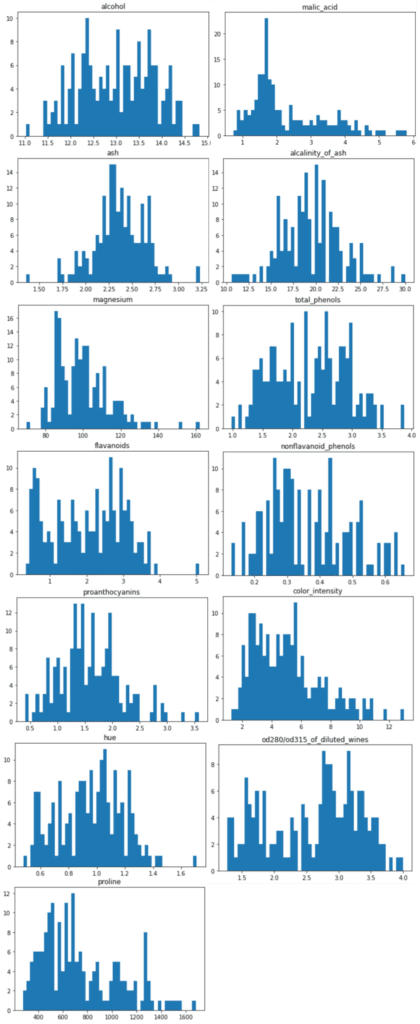
Histogram Distribution
Data with variance is the data that is worth paying attention to. So let’s actually visualize the distribution of the data.
Seeing is believing!
We can perform the histogram plotting by “plt.hist()” in “matplotlib”, a famous library for visualization. The argument “bins” can control the fineness of plot.
for name in f.columns:
plt.title(name)
plt.hist(f[name], bins=50)
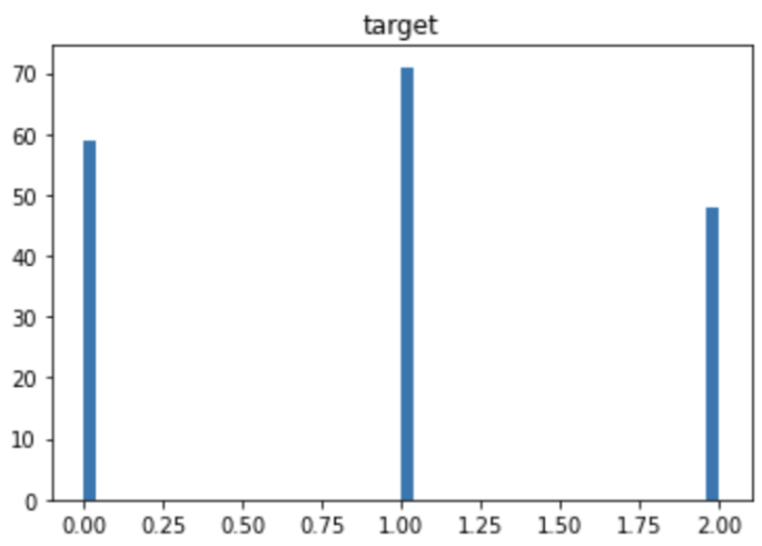
plt.show()The distribution of the target variable is as follows. You can see that each category has almost the same amount of data. If the number of data is biased by category, you should pay attention to the decrease in accuracy due to imbalance.
The distributions of the explanatory variables are below. We can see the difference in variance between the explanatory variables.
Summary
We have seen how to perform EDA briefly. The purpose of EDA is to properly identify the nature of the dataset. Proper EDA can make it possible to explore the next step effectively, e.g. feature engineering and modeling methods.
In the case of classification problems, principal component analysis can be considered as a deeper analysis method. I will introduce it in another post.