Category: Pandas

The descriptive statistics have important information because they reflect a summary of a dataset. For example, from descriptive statistics, we can know the scale, variation, minimum and maximum values. If you know the above information, you can have a sense of grasping whether one of the data is large or small, or whether it deviates greatly from the average value.

In this post, we will see the descriptive statistics with a definition. Understanding statistical descriptions not only helps to develop a sense of a dataset but is also useful for understanding the preprocessing of a dataset.

The complete notebook can be found on GitHub.

Dataset

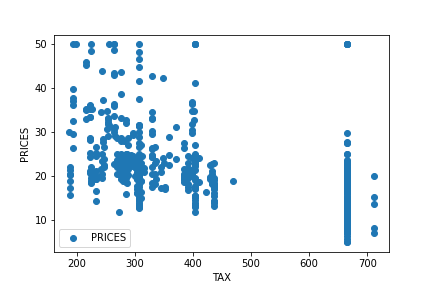
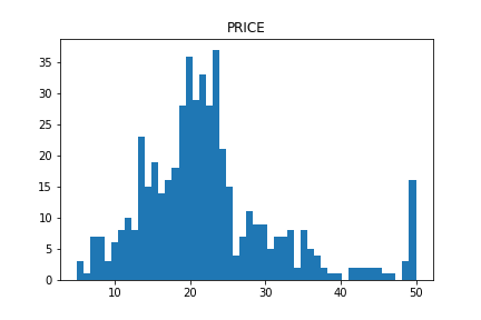
Here, we utilize the Boston house prices dataset for calculating the descriptive statistics, such as mean, variance, and standard deviation. The reason why we adopt this dataset is we can use it so easily with the scikit-learn library.

The code for using the dataset as Pandas DataFrame is as follows.

import numpy as np              ##-- Numpy
import pandas as pd             ##-- Pandas
import sklearn                  ##-- Scikit-learn
import matplotlib.pylab as plt  ##-- Matplotlib

from sklearn.datasets import load_boston
dataset = load_boston()

df = pd.DataFrame(dataset.data)
df.columns = dataset.feature_names
df["PRICES"] = dataset.target
df.head()

>>       CRIM   ZN  INDUS  CHAS  NOX   RM   AGE	 DIS  RAD	TAX PTRATIO	  B   LSTAT PRICES
>>  0   0.00632 18.0  2.31  0.0 0.538 6.575 65.2  4.0900  1.0 296.0 15.3  396.90  4.98  24.0
>>  1	0.02731	 0.0  7.07  0.0 0.469 6.421 78.9  4.9671  2.0 242.0 17.8  396.90  9.14  21.6
>>  2	0.02729	 0.0  7.07  0.0 0.469 7.185 61.1  4.9671  2.0 242.0 17.8  392.83  4.03  34.7
>>  3	0.03237	 0.0  2.18  0.0 0.458 6.998 45.8  6.0622  3.0 222.0 18.7  394.63  2.94  33.4
>>  4	0.06905	 0.0  2.18  0.0 0.458 7.147 54.2  6.0622  3.0 222.0 18.7  396.90  5.33  36.2

The details of this dataset are introduced in another post below. In this post, let’s calculate the mean, the variance, the standard deviation for “df[“PRICES”]”, the housing prices.

Mean

The mean $\mu$ is the average of the data. It must be one of the most familiar concepts. However, the concept of mean is important because we can obtain the sense of whether one value of data is large or small. Such a feeling is important for a data scientist.

Now, assuming that $N$ data are $x_{1}$, $x_{2}$, …, $x_{n}$, the mean $\mu$ is defined by the following formula.
$$\begin{eqnarray*}
\mu
=
\frac{1}{N}
\sum^{N}_{i=1}
x_{i}
,
\end{eqnarray*}$$
where $x_{i}$ is the value of $i$-th data.

It may seem a little difficult when expressed in mathematical symbols. However, as you know, we just take a summation of all the data and divide it by the number of data. Once we defined the mean, we can define the variance.

Then, let’s calculate the mean of each column. We can easily calculate by the “mean()” method.

df.mean()

>>  CRIM         3.613524
>>  ZN          11.363636
>>  INDUS       11.136779
>>  CHAS         0.069170
>>  NOX          0.554695
>>  RM           6.284634
>>  AGE         68.574901
>>  DIS          3.795043
>>  RAD          9.549407
>>  TAX        408.237154
>>  PTRATIO     18.455534
>>  B          356.674032
>>  LSTAT       12.653063
>>  PRICES      22.532806
>>  dtype: float64

When you want the mean value of just one column, for example the “PRICES”, the code is as follows.

df["PRICES"].mean()

>>  22.532806324110677

Variance

The variance $\sigma^{2}$ reflects the dispersion of data from the mean value. The definition is as follows.

$$\begin{eqnarray*}
\sigma^{2}
=
\frac{1}{N}
\sum^{N}_{i=1}
\left(
x_{i} – \mu
\right)^{2},
\end{eqnarray*}$$

where $N$, $x_{i}$, and $\mu$ are the number of the data, the value of $i$-th data, and the mean of $x$, respectively.

Expressed in words, the variance is the mean of the squared deviations from the mean of the data. It is no exaggeration to say that the information in the data exists in a variance! In other words, there is no worth to pay an attention to the data with the ZERO variance.

For example, let’s consider predicting math skills from exam scores. The exam scores of the person(A, B, and C) are like the below table.

From the above table, we can clearly see that those who are good at physics are also good at math. On the other hand, it is impossible to infer whether the person is good at mathematics from chemistry scores. Because all three scores equal the average score of 60. Namely, the variance of chemistry is ZERO!! This fact indicates that the scores of chemistry have no information, no worth to pay attention to. We should drop the “Chemistry” columns from the dataset when analyzing! This is one of the data preprocessing.

Then, let’s calculate the mean of each column of the Boston house prices dataset. We can easily calculate by the “var()” method.

df.var()

>>  CRIM          73.986578
>>  ZN           543.936814
>>  INDUS         47.064442
>>  CHAS           0.064513
>>  NOX            0.013428
>>  RM             0.493671
>>  AGE          792.358399
>>  DIS            4.434015
>>  RAD           75.816366
>>  TAX        28404.759488
>>  PTRATIO        4.686989
>>  B           8334.752263
>>  LSTAT         50.994760
>>  PRICES        84.586724
>>  dtype: float64

Standard Deviation

The standard deviation $\sigma$ is defined by the root of the variance as follows.

$$\begin{eqnarray*}
\sigma
=
\sqrt{
\frac{1}{N}
\sum^{N}_{i=1}
\left(
x_{i} – \mu
\right)^{2}
},
\end{eqnarray*}$$

where $N$, $x_{i}$, and $\mu$ are the number of the data, the value of $i$-th data, and the mean of $x$, respectively.

Why we introduced the standard deviation instead of the variance? This is because the unit becomes the same when we adopt the standard deviation of $\sigma$. Then, we can recognize $\sigma$ as the variation from the mean.

Then, let’s calculate the standard deviation of each column of the Boston house prices dataset. We can easily calculate by the “std()” method.

df.std()

>> CRIM         8.601545
>> ZN          23.322453
>> INDUS        6.860353
>> CHAS         0.253994
>> NOX          0.115878
>> RM           0.702617
>> AGE         28.148861
>> DIS          2.105710
>> RAD          8.707259
>> TAX        168.537116
>> PTRATIO      2.164946
>> B           91.294864
>> LSTAT        7.141062
>> PRICES       9.197104
>> dtype: float64

In fact, at the stage of defining these three concepts, we can define the Gaussian distribution. However, I’ll introduce the Gaussian distribution in another post.

Other descriptive statistics are calculated in the same way, so carefully select the ones you use most often and list them below.

Confirm all at once

Pandas has the useful function “describe()”, which describes the basic descriptive statistics. The “describe()” method is very convenient to use as a starting point.

df.describe()

>>         CRIM        ZN          INDUS       CHAS        NOX         RM          AGE         DIS         RAD         TAX         PTRATIO     B           LSTAT       PRICES
>>  count  506.000000  506.000000  506.000000  506.000000  506.000000  506.000000  506.000000  506.000000  506.000000  506.000000  506.000000  506.000000  506.000000  506.000000
>>  mean     3.613524   11.363636   11.136779    0.069170    0.554695    6.284634   68.574901    3.795043    9.549407  408.237154   18.455534  356.674032   12.653063  22.532806
>>  std      8.601545   23.322453    6.860353    0.253994    0.115878    0.702617   28.148861    2.105710    8.707259  168.537116    2.164946   91.294864    7.141062  9.197104
>>  min      0.006320    0.000000    0.460000    0.000000    0.385000    3.561000    2.900000    1.129600    1.000000  187.000000   12.600000    0.320000    1.730000  5.000000
>>  25%      0.082045    0.000000    5.190000    0.000000    0.449000    5.885500   45.025000    2.100175    4.000000  279.000000   17.400000  375.377500    6.950000  17.025000
>>  50%      0.256510    0.000000    9.690000    0.000000    0.538000    6.208500   77.500000    3.207450    5.000000  330.000000   19.050000  391.440000   11.360000  21.200000
>>  75%      3.677083   12.500000   18.100000    0.000000    0.624000    6.623500   94.075000    5.188425   24.000000  666.000000   20.200000  396.225000   16.955000  25.000000
>>  max     88.976200  100.000000   27.740000    1.000000    0.871000    8.780000  100.000000   12.126500   24.000000  711.000000   22.000000  396.900000   37.970000  50.000000

Note that,

“count”: Number of the data for each columns
“25%”: Value at the 25% position of the data
“50%”: Value at the 50% position of the data, equaling to “Median”
“75%”: Value at the 25% position of the data

Summary

We have seen the brief explanation of the basic descriptive statistics and how to calculate them. Understanding the concept of descriptive statistics is essential to understand the dataset. You should note the fact in your memory that the information of the dataset is included in the descriptive statistics.

The author hopes this blog helps readers a little.

Linear regression is one of the basic techniques for machine learning analyses. You may know, in general, other methods are often superior to linear regression in terms of prediction accuracy. However, linear regression has the advantage that the model is simple and high interpretable.

For a data scientist, to understand a dataset is highly important. Therefore, linear regression plays a powerful role as a first step for the purpose of understanding the dataset first.

In this post, we will see the process of a linear regression analysis against the Boston house prices dataset. The author will explain with the step-by-step guide in mind !!

What is a Linear Regression?

Linear regression is based on the assumption of the linar relationship between a target variable and independent variables. Then, if you can represent your dataset well, you can expect a proportional relationship between the independent and objective variables.

In the mathematical expression, the representation of a linear regression is as follows.

$$y =\omega_{0}+\omega_{1}x_{1}+\omega_{2}x_{2}+…+\omega_{N}x_{N},$$

where $y$, $x_{i}$, and $\omega_{i}$ are a target variable, an independent variable, and a coefficient, respectively.

The details of the theory are explained in another post below.

Also, for reference, another post provides an example of linear regression with short code.

From here, let’s perform a linear regression analysis on the Boston house prices dataset!

Prepare the Dataset

In this analysis, we adopt the Boston house prices dataset, one of the famous open datasets published by the StatLib library which is maintained at Carnegie Mellon University. This is because we can use this dataset so easily. Just load from the scikit-learn library without downloading the file.

from sklearn.datasets import load_boston
dataset = load_boston()

The details of the Boston house prices dataset is introduced in another post. But, you can understand the following analysis without referring.

Confirm the Dataset as Pandas DataFrame

Here, we get 3 types of data from “dataset”, described below, as the Pandas DataFrame.

dataset.data: values of the explanatory variables
dataset.target: values of the target variable (house prices)
dataset.feature_names: the column names

import pandas as pd

f = pd.DataFrame(dataset.data)
f.columns = dataset.feature_names
f["PRICES"] = dataset.target
f.head()

>>       CRIM   ZN  INDUS  CHAS  NOX   RM   AGE	 DIS  RAD	TAX PTRATIO	  B   LSTAT PRICES
>>  0   0.00632 18.0  2.31  0.0 0.538 6.575 65.2  4.0900  1.0 296.0 15.3  396.90  4.98  24.0
>>  1	0.02731	 0.0  7.07  0.0 0.469 6.421 78.9  4.9671  2.0 242.0 17.8  396.90  9.14  21.6
>>  2	0.02729	 0.0  7.07  0.0 0.469 7.185 61.1  4.9671  2.0 242.0 17.8  392.83  4.03  34.7
>>  3	0.03237	 0.0  2.18  0.0 0.458 6.998 45.8  6.0622  3.0 222.0 18.7  394.63  2.94  33.4
>>  4	0.06905	 0.0  2.18  0.0 0.458 7.147 54.2  6.0622  3.0 222.0 18.7  396.90  5.33  36.2

Let’s try to check the correlation between only “PRICES” and “TAX”.

import matplotlib.pylab as plt  #-- "Matplotlib" for Plotting

f.plot(x="TAX", y="PRICES", style="o")
plt.ylabel("PRICES")
plt.show()

At first glance, there seems to be no simple proportional relationship. Including other variables, the EDA(Exploratory data analysis) for this dataset is introduced in another post.

Pick up the Variables we use

Explicitly define the variables to use for getting from the data frame.

TargetName = "PRICES"
FeaturesName = [\
              #-- "Crime occurrence rate per unit population by town"
              "CRIM",\
              #-- "Percentage of 25000-squared-feet-area house"
              'ZN',\
              #-- "Percentage of non-retail land area by town"
              'INDUS',\
              #-- "Index for Charlse river: 0 is near, 1 is far"
              'CHAS',\
              #-- "Nitrogen compound concentration"
              'NOX',\
              #-- "Average number of rooms per residence"
              'RM',\
              #-- "Percentage of buildings built before 1940"
              'AGE',\
              #-- 'Weighted distance from five employment centers'
              "DIS",\
              ##-- "Index for easy access to highway"
              'RAD',\
              ##-- "Tax rate per $100,000"
              'TAX',\
              ##-- "Percentage of students and teachers in each town"
              'PTRATIO',\
              ##-- "1000(Bk - 0.63)^2, where Bk is the percentage of Black people"
              'B',\
              ##-- "Percentage of low-class population"
              'LSTAT',\
              ]

Get from the data frame into “X” and “Y”.

X = f[FeaturesName]
Y = f[TargetName]

Standardize the Variables

For numerical variables, we should standardize because the scales of variables are different.

In mathematically, the definition of the conversion of standardization is as follows.

$$\begin{eqnarray*}
\tilde{x}=
\frac{x-\mu}{\sigma}
,
\end{eqnarray*}$$

where $\mu$ and $\sigma$ are the mean and the standard deviation, respectively.

Execution code by scikit-learn is just 4 line code as follows.

from sklearn import preprocessing
sscaler = preprocessing.StandardScaler()
sscaler.fit(X)
X_std = sscaler.transform(X)

Regarding standardization, the details are explained in another post. The standardization is an important preprocessing for numerical variables. If you don’t know standardization, the author recommends that you check the details once.

Split the Dataset

Here, we split the dataset into the train data and the test data. Why we have to split? This is because we must evaluate the generalization performance of the model against unknown data.

You can see that the above idea is valid because our purpose is to predict new data.

Then, let’s split the dataset. Of course, it is easy with scikit-learn!

from sklearn.model_selection import train_test_split
X_train, X_test, Y_train, Y_test = train_test_split(X_std, Y, test_size=0.2, random_state=99)

We pass the dataset “(X_std, Y)” to the “train_test_split()” function. The rate of the train data and the test data is defined by the argument “test_size”. Here, the rate is set to be “8:2”. And, “random_state” are set for reproducibility. You can use any number. The author often uses “99” because “99” is my favorite NFL player’s uniform number!

At this point, data preparation and preprocessing are fully completed!
Finally, we can perform the linear regression analysis!

Create an Instance for Linear Regression

Here, let’s create the model for linear regression. We can perform with the just 3 line code. The role of each line is as follows.

1. Import the “LinearRegression()” function from scikit-learn
2. Create the model as an instance “regressor” by “LinearRegression()”
3. Train the model “regressor” with train data “(X_train, Y_train)”

from sklearn.linear_model import LinearRegression
regressor = LinearRegression()
regressor.fit(X_train, Y_train)

Predict the train and test data

To check the performance of the model, we get the predicted values for the train and test data.

y_pred_train = regressor.predict(X_train)
y_pred_test = regressor.predict(X_test)

Then, let’s visualize the result by matplotlib.

import seaborn as sns

plt.figure(figsize=(5, 5), dpi=100)
sns.set()
plt.xlabel("PRICES")
plt.ylabel("Predicted PRICES")
plt.xlim(0, 60)
plt.ylim(0, 60)
plt.scatter(Y_train, y_pred_train, lw=1, color="r", label="train data")
plt.scatter(Y_test, y_pred_test, lw=1, color="b", label="test data")
plt.legend()
plt.show()

About the above figure, the red and blue circles show the results of the train and test data, respectively. We can see that the prediction accuracy decreases as the price increases.

Here, we check $R^{2}$ score, the coefficient of determination. $R^{2}$ is the index for how much the model is fitted to the dataset. When $R^{2}$ is close to $1$, the model accuracy is good. Conversely, when $R^{2}$ approaches $0$, it means that the model accuracy is poor.

We can calculate $R^{2}$ by the “r2_score()” function in scikit-learn.

from sklearn.metrics import r2_score
R2 = r2_score(Y_test, y_pred_test)
R2

>>  0.6674690355194665

The score $0.67$ is not bad, but also not good.

How to Improve the Score?

Here, one easy way to improve your score is introduced. The answer is to convert the target variable “PRICES” to a logarithmic scale. Converting to a logarithmic scale reduces the effect of errors in the high “PRICES” range. Reducing the effect of errors between the train data and the predicted values leads to improved models. Logarithmic conversion techniques are often simple and effective and should be helpful to remember.

Then, let’s try!

First, converting the target variable “PRICES” to a logarithmic scale.

##-- Logarithmic scaling
Y_log = np.log(Y)

Next, we split the dataset again.

from sklearn.model_selection import train_test_split
X_train, X_test, Y_train, Y_test = train_test_split(X_std, Y_log, test_size=0.2, random_state=99)

And, retrain the model and predict again.

regressor.fit(X_train, Y_train)
y_pred_train = regressor.predict(X_train)
y_pred_test = regressor.predict(X_test)

Plot the result again as follows. Note that the predicted value is the value after logarithmic conversion, so it must be inversely converted by “np.ep()” when plotting.

import numpy as np

plt.figure(figsize=(5, 5), dpi=100)
sns.set()
plt.xlabel("PRICES")
plt.ylabel("Predicted PRICES")
plt.xlim(0, 60)
plt.ylim(0, 60)
plt.scatter(np.exp(Y_train), np.exp(y_pred_train), lw=1, color="r", label="train data")
plt.scatter(np.exp(Y_test), np.exp(y_pred_test), lw=1, color="b", label="test data")
plt.legend()
plt.show()

It may be hard to see the improvement from the figure, but when you compare $R^{2}$, you can see that it has improved clearly.

R2 = r2_score(Y_test, y_pred_test)
R2

>>  0.7531747761424288

$R^{2}$ has improved from 0.67 to 0.75!

Summary

We have seen how to perform the linear regression analysis against the Boston house prices dataset. The basic approach to regression analysis is as described here. So, we can apply this approach to other datasets.

Note that the important thing is to have a good understanding of the dataset, making it possible to perform an analysis reflecting the essence.

Certainly, there are several methods that can be expected to be more accurate, such as random forest and neural net. However, linear regression analysis can be a good first step to understanding datasets deeper.

The author hopes this blog helps readers a little.