Category: PyCaret

PyCaret is a useful auto ML python library because we can deploy machine learning models with low codes. We can also perform preprocessing, compare models, and tune hyperparameters, of course with low codes.

Recently, PyCaret version 2.3.6 was released. This is big news because several new wonderful functions were implemented in this release version! The details are described in this article written by PyCaret creator.

In this article, we will check the summary of this release. And, the three new features will be introduced.

New Features

• Dashboard: interactive dashborad for a trained model.
• EDA: Explonatory Data Analysis
• Convert Model: converting a trained model from python into other programing language, such as C, Java, Go, JavaScript, Visual Basic, C#, PowerShell, R, PHP, Dart, Haskell, Ruby, F#.
• Fairness
• Web API based on FastAPI
• Create Dockerfile and requirements file for a API
• Web Application based on Gradio
• Monitor Data Drift
• Optimize Threshold for classification
• New Documentation

As seeing the above new feature list, PyCaret is evolving dramatically!

In the following, we will introduce some of the new functions using normal regression analysis as an example.

Installation

If you have NOT installed PyCaret yet, you can easily install it by the following command. Note that specify the PyCaret version!

$pip install pycaret==2.3.6

From here, the sample code in this post is supposed to run on Jupyter Notebook.

Import Libraries

In advance, we load all the modules for regression analysis of PyCaret.

from pycaret.regression import *

Dataset

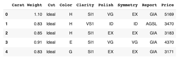
We use the diamond dataset for regression analysis.

# load dataset
from pycaret.datasets import get_data

df = get_data('diamond')

Set up the environment by the “setup()” function

PyCaret needs to initialize an environment by the “setup()” function. Conveniently, PyCaret infers the data type of the variables in the dataset.

Arguments of setup() are the dataset as Pandas DataFrame, the target-column name, and the “session_id”. The “session_id” equals a random seed.

s = setup(df, target='Price', session_id = 20220121)

Create a Model

Due to the simplicity of the technique and the interpretability of the model, we will adopt lr(Linear Regression) for the models that will be used below.

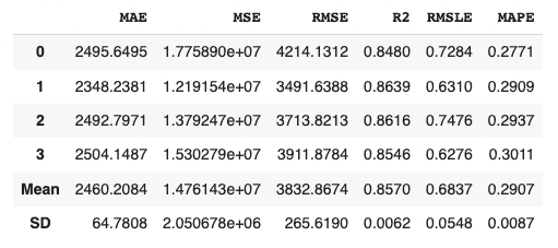
We can create the selected model by create_model() with the argument of “lr”. Another argument of “fold” is the number of cross-validation. “fold = 4” indicates we split the dataset into four and train the model in each dataset separately.

lr = create_model("lr", fold=4)

Introduction of New Features of PyCaret 2.3.6

From here, we will introduce two of the new features.

Convert model

With this new function, we can convert a trained model into another language, e. g. from python to C. This function is very useful when operating the created model.

Note that we need to install the dependency libraries.

$pip install m2cgen

Then, we can convert a model.

model_c = convert_model(model, language='c')
print(model_c)

Create Web App

This new function requires the “gradio” library.

$pip install gradio

Just 1 line code. We can create a web app.

create_app(model)

Summary

We have seen the new features of PyCaret 2.3.6.

In this article, we saw covering the model into another language and creating a web app.

Just 1 line.

Wouldn’t it be great? If you sympathize with it, please give it a try.

The author hopes this blog helps readers a little.

PyCaret is a useful auto ML python library because we can deploy machine learning models with low codes. We can also perform preprocessing, compare models, and tune hyperparameters, of course with low codes.

Recently, PyCaret version 2.3.6 was released. This is big news because several new wonderful functions were implemented in this release version! The details are described in this article written by PyCaret creator.

In this article, we will check the summary of this release. And, the three new features will be introduced.

New Features

• Dashboard: interactive dashborad for a trained model.
• EDA: Explonatory Data Analysis
• Convert Model: converting a trained model from python into other programing language, such as C, Java, Go, JavaScript, Visual Basic, C#, PowerShell, R, PHP, Dart, Haskell, Ruby, F#.
• Fairness
• Web API based on FastAPI
• Create Dockerfile and requirements file for a API
• Web Application based on Gradio
• Monitor Data Drift
• Optimize Threshold for classification
• New Documentation

As seeing the above new feature list, PyCaret is evolving dramatically!

In the following, we will introduce some of the new functions using normal regression analysis as an example.

Installation

If you have NOT installed PyCaret yet, you can easily install it by the following command. Note that specify the PyCaret version!

$pip install pycaret==2.3.6

From here, the sample code in this post is supposed to run on Jupyter Notebook.

Import Libraries

In advance, we load all the modules for regression analysis of PyCaret.

from pycaret.regression import *

Dataset

We use the diamond dataset for regression analysis.

# load dataset
from pycaret.datasets import get_data

df = get_data('diamond')

Set up the environment by the “setup()” function

PyCaret needs to initialize an environment by the “setup()” function. Conveniently, PyCaret infers the data type of the variables in the dataset.

Arguments of setup() are the dataset as Pandas DataFrame, the target-column name, and the “session_id”. The “session_id” equals a random seed.

s = setup(df, target='Price', session_id = 20220121)

Create a Model

Due to the simplicity of the technique and the interpretability of the model, we will adopt lr(Linear Regression) for the models that will be used below.

We can create the selected model by create_model() with the argument of “lr”. Another argument of “fold” is the number of cross-validation. “fold = 4” indicates we split the dataset into four and train the model in each dataset separately.

lr = create_model("lr", fold=4)

Introduction of New Features of PyCaret 2.3.6

From here, we will introduce two of the new features.

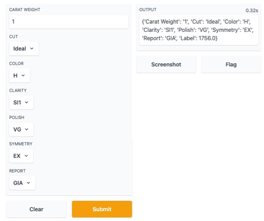
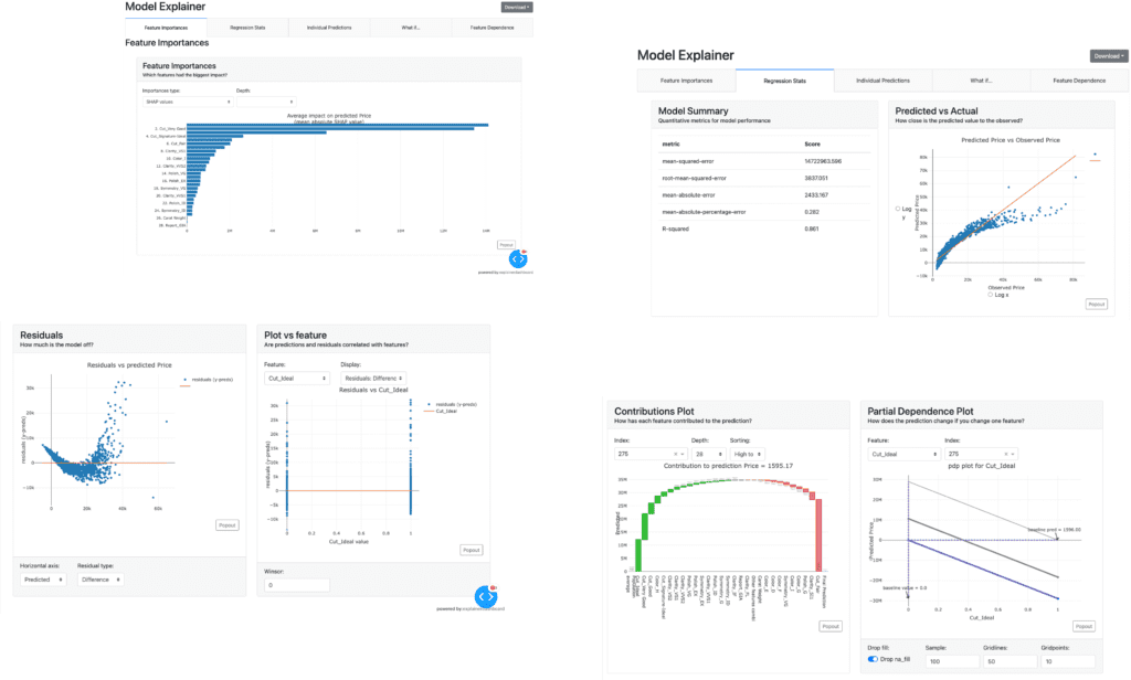
Dashboard

With this new function, we can create a dashboard for a trained model.

The dashboard function is implemented by ExplainerDashboard, we need the “explainerdashboard” library. We can install it with the pip command.

$pip install explainerdashboard

Then, we can create a dashboard.

dashboard(model)

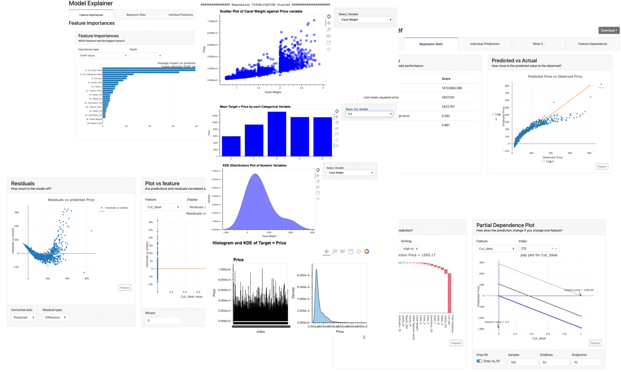
Parts of the dashboard screen are introduced in the figure below.

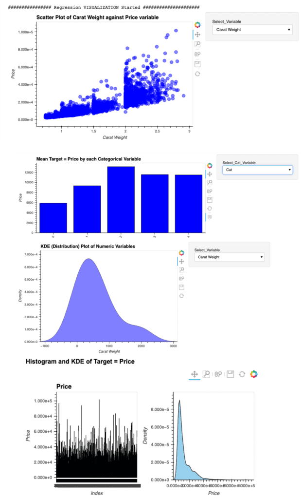
EDA(Exploratory Data Analysis)

This new function requires the “autoviz” library.

$pip install autoviz

Just 1 line code. We can perform the EDA.

eda()

Summary

We have seen the new features of PyCaret 2.3.6.

In this article, we saw the Dashboard and EDA function.

Just 1 line.

We can create a dashboard and perform the EDA of a trained model. Wouldn’t it be great? If you sympathize with it, please give it a try.

The author hopes this blog helps readers a little.

In this post, we will learn the tutorial of PyCaret from the regression problem; prediction of diabetes progression. PyCaret is so useful especially when you start to tackle a machine learning problem such as regression and classification problems. This is because PyCaret makes it easy to perform preprocessing, comparing models, hyperparameter tuning, and prediction.

Requirement

PyCaret is now highly developed, so you should check the version of the library.

pycaret == 2.2.3
pandas == 1.1.5
scikit-learn == 0.23.2
matplotlib == 3.2.2

If you have NOT installed PyCaret yet, you can easily install it by the following command on your terminal or command prompt.

$pip install pycaret

Or you can specify the version of PyCaret.

$pip install pycaret==2.2.3

From here, the sample code in this post is supposed to run on Jupyter Notebook.

Import Library

##-- PyCaret
import pycaret
from pycaret.regression import *
##-- Pandas
import pandas as pd
from pandas import Series, DataFrame
##-- Scikit-learn
import sklearn

Load dataset

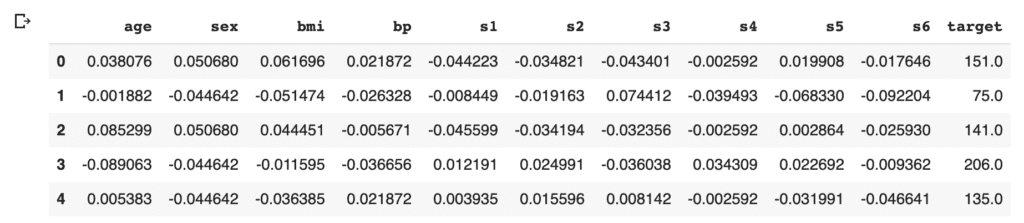
In this post, we use “the diabetes dataset” from scikit-learn library. This dataset is easy to use because we can load this dataset from the scikit-learn library, NOT from the external file.

We will predict a quantitative measure of diabetes progression one year after baseline. So, the target variable is diabetes progression in “dataset.target“. And, there are ten explanatory variables (age, sex, body mass index, average blood pressure, and six blood serum measurements).

First, load the dataset from “load_diabetes()” as “dataset”. And, for convenience, convert the dataset into the pandas-DataFrame form.

from sklearn.datasets import load_diabetes
dataset = load_diabetes()

df = pd.DataFrame(dataset.data)

It should be noted that we can confirm the description of the dataset.

print(dataset.DESCR)

An excerpt of the explanation of the explanatory variables is as follows.

:Attribute Information:
    - age     age in years
    - sex
    - bmi     body mass index
    - bp      average blood pressure
    - s1      tc, T-Cells (a type of white blood cells)
    - s2      ldl, low-density lipoproteins
    - s3      hdl, high-density lipoproteins
    - s4      tch, thyroid stimulating hormone
    - s5      ltg, lamotrigine
    - s6      glu, blood sugar level    

Then, we assign the above names of the columns to the data frame of pandas. And, we create the “target” column, i.s., the prediction target, and assign the supervised values.

df.columns = dataset.feature_names
df["target"] = dataset.target
df.head()

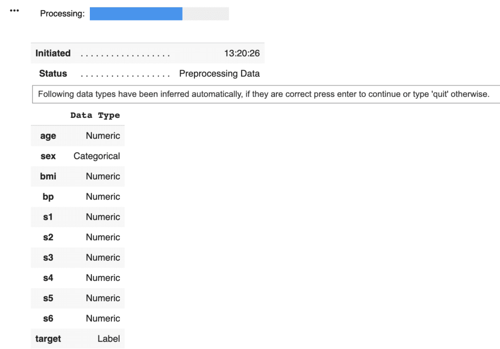
Here, we devide the dataset into train- and test- datasets, making it possible to check the ability of the trained model against an unseen data. We split the dataset into train and test datasets, as 8:2.

split_rate = 0.8
data = df.iloc[ : int(split_rate*len(df)), :]
data_pre = df.iloc[ int(split_rate*len(df)) :, :]

Set up the environment by the “setup()” function

PyCaret needs to initialize an environment by the “setup()” function. Conveniently, PyCaret infers the data type of the variables in the dataset. Due to regression analysis, let’s leave only the numerical data. Namely, we delete the categorical variables. This approach would be practical as a first analysis to understand the dataset.

Arguments of setup() are the dataset as Pandas DataFrame, the target-column name, and the “session_id”. The “session_id” equals a random seed.

model = setup(data = data, target = "target", session_id=99)

PyCaret told us that just “sex” is a categorical variable. Then, we drop its columns and reset up.

data = data.drop('sex', 1) # "1" indicate the columns.
model = setup(data = data, target = "target", session_id=99)

Compare models

We can easily compare models between different machine-learning methods. It is so practical just to know which is more effective, the regression model or the decision tree model.

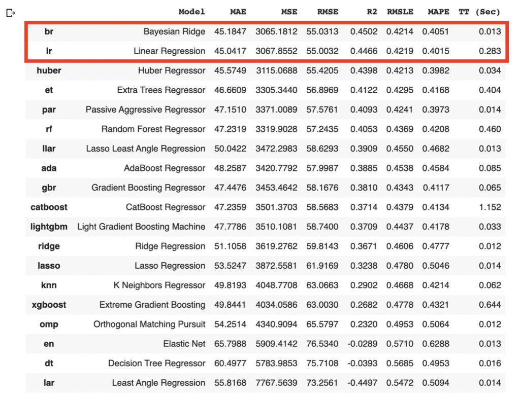
compare_models()

As the above results, the br(Bayesian Ridge) and lr(Linear Regression) have the highest accuracies in the above models. In general, there is a tendency that a decision tree method realizes a higher accuracy than that of a regression method. However, from the viewpoint of model interpretability, the regression method is more effective than the decision tree method, especially when the accuracy is almost the same. Regression analysis tends to be easy to provide insight into the dataset.

Due to the simplicity of the technique and the interpretability of the model, we will adopt lr(Linear Regression) for the models that will be used below. The details of the linear regression technique are described in another post below.

Select and Create the model

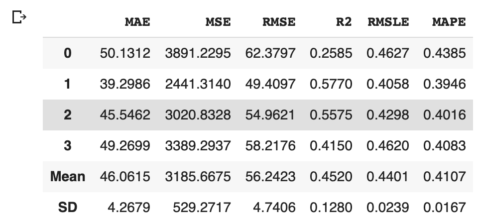
We can create the selected model by create_model() with the argument of “lr”. Another argument of “fold” is the number of cross-validation. “fold = 4” indicates we split the dataset into four and train the model in each dataset separately.

lr = create_model("lr", fold=4)

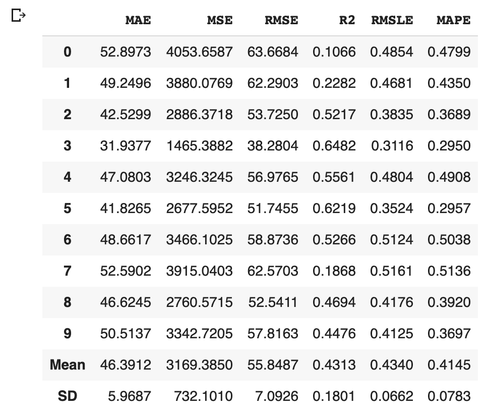
Optimize Hyperparameters

PyCaret makes it possible to optimize the hyperparameters. Just you pass the object cerated by create_model() to tune_model(). Note that optimization is done by the random grid-search technique.

Predict the test data

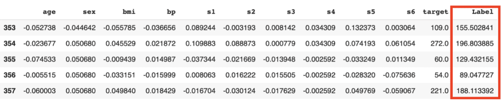
Let’s predict the test data by the above model. We can do it easily with just one sentence.

predictions = predict_model(tuned_model, data=data_pre)
predictions.head()

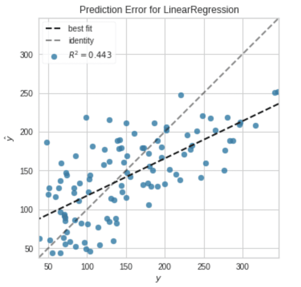
The added column, “Label”, is the predicted values. Besides, we can confirm the famous metric, such as $R^2$.

from pycaret.utils import check_metric
check_metric(predictions["target"], predictions["Label"], 'R2')

>>  0.535

Visualization

It is also easy to visualize the results.

plot_model(tuned_model, plot = 'error')

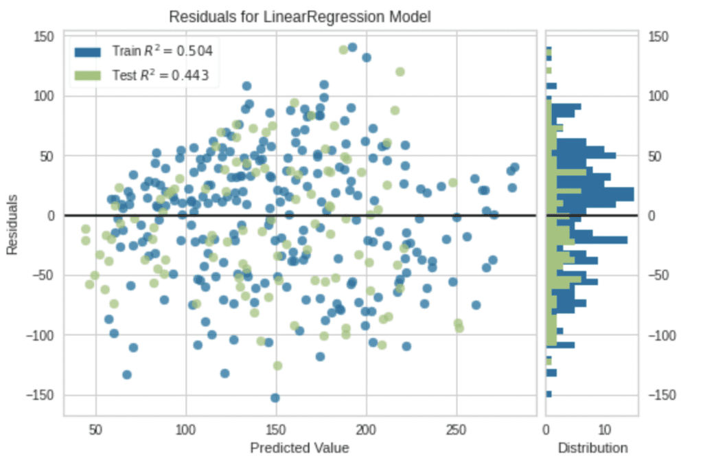
Note that, without an argument, a residual plot will be visualized.

plot_model(tuned_model)

Summary

We have seen the tutorial of PyCaret from the regression problem. PyCaret is so useful to perform the first analysis against the unknown dataset.

In data science, it is important to try various approaches and to repeat small trials quickly. Therefore, there might be worth using PyCaret to do such thing more efficiently.

The author hopes this blog helps readers a little.