The machine learning approaches, such as decision-tree-based methods and linear regression, have been already introduced in other posts. These approaches are practical in real data science tasks.
However, deep learning approaches are also essential skills for a data scientist. In real, deep learning would be a more powerful approach when a dataset is larger than that of Boston house prices.
In this post, we will see a brief description of how to apply a neural network to the Boston house prices dataset.
Related posts are below. Please refer to those.
Import liraries
from sklearn.datasets import load_boston
from sklearn import preprocessing
from sklearn.metrics import r2_score
import pandas as pd
import numpy as np
import matplotlib.pylab as plt
import seaborn as sns
sns.set()
import torch
import torch.nn as nn
import torch.nn.functional as F
import torch.optim as optim
Load the Dataset
In this post, we use the Boston house prices dataset in the scikit-learn library. We can easily load the dataset by just two lines below.
# from sklearn.datasets import load_boston
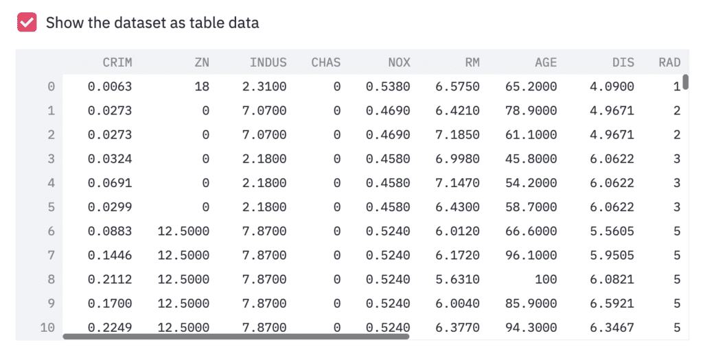
dataset = load_boston()Read the Dataset as Pandas DataFrame
# import pandas as pd
df = pd.DataFrame(dataset.data)
df.columns = dataset.feature_names
df["PRICES"] = dataset.target
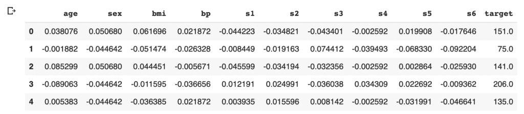
df.head()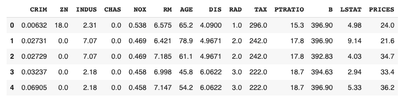
Example: RM vs PRICES
Let’s try to check the correlation between only “PRICES” and “RM”.
# import matplotlib.pylab as plt
f.plot(x="RM", y="PRICES", style="o")
plt.ylabel("PRICES")
plt.show()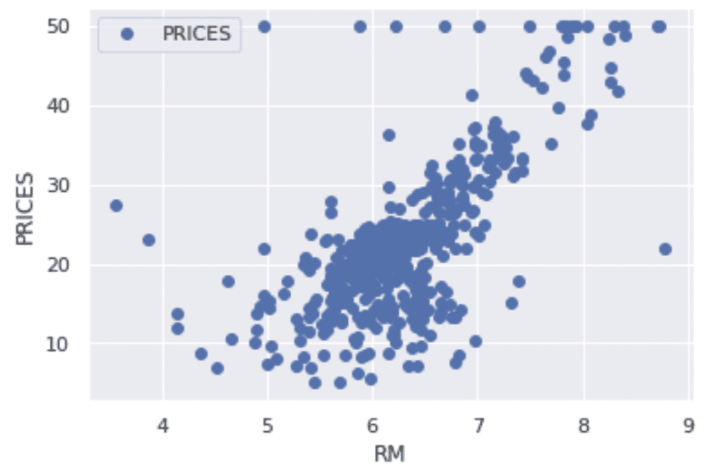
Variables to be used
TargetName = "PRICES"
FeaturesName = [
#-- "Crime occurrence rate per unit population by town"
"CRIM",
#-- "Percentage of 25000-squared-feet-area house"
'ZN',
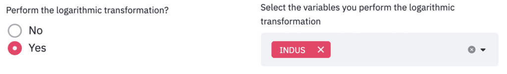
#-- "Percentage of non-retail land area by town"
'INDUS',
#-- "Index for Charlse river: 0 is near, 1 is far"
'CHAS',
#-- "Nitrogen compound concentration"
'NOX',
#-- "Average number of rooms per residence"
'RM',
#-- "Percentage of buildings built before 1940"
'AGE',
#-- 'Weighted distance from five employment centers'
"DIS",
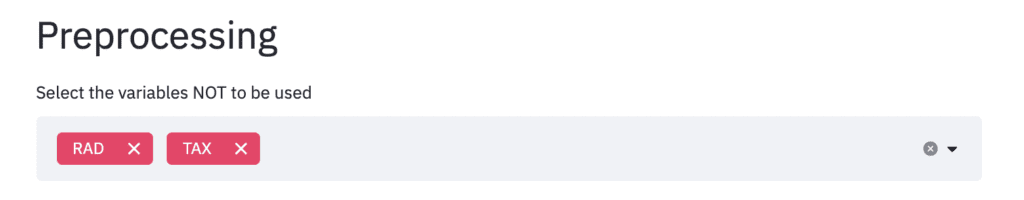
##-- "Index for easy access to highway"
'RAD',
##-- "Tax rate per $100,000"
'TAX',
##-- "Percentage of students and teachers in each town"
'PTRATIO',
##-- "1000(Bk - 0.63)^2, where Bk is the percentage of Black people"
'B',
##-- "Percentage of low-class population"
'LSTAT',
]We prepare the input and target variables as “X” and “Y”.
X = f[FeaturesName]
Y = f[TargetName]
Standardize the Variables
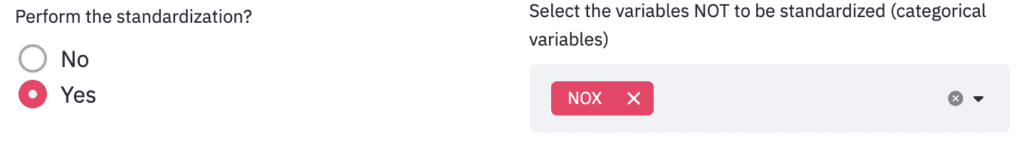
We need to standardize or normalize the numerical variable in neural network analysis. This is because the magnitude of each variable affects its scale of parameters in a neural network. Therefore, the difference in the scale of the variables would make training of the model difficult.
From the above reason, we perform the standardization into the variables. In mathematically, the definition of the conversion of standardization is as follows.
$$\begin{eqnarray*}
\tilde{x}=
\frac{x-\mu}{\sigma}
,
\end{eqnarray*}$$
where $\mu$ and $\sigma$ are the mean and the standard deviation, respectively.
# from sklearn import preprocessing
sscaler = preprocessing.StandardScaler()
sscaler.fit(X)
X_std = sscaler.transform(X)Split the Dataset
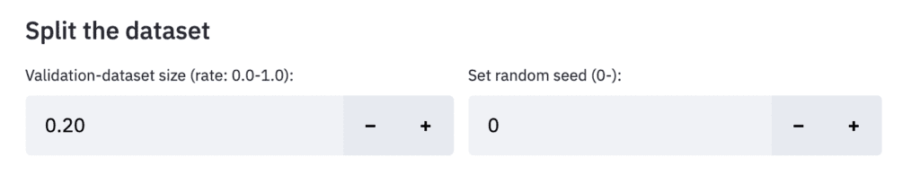
To validate the performance of the trained model against unseen data, we have to split the dataset into the train data and the test data.
We pass the dataset “(X, Y)” to the “train_test_split()” function. The rate of the train data and the test data is defined by the argument “test_size”. Here, the rate is set to be “8:2”. And, “random_state” is set for reproducibility. You can use any number.
# from sklearn.model_selection import train_test_split
X_train, X_test, Y_train, Y_test = train_test_split(X_std, Y, test_size=0.2, random_state=99)
Define a Neural network model by PyTorch
We define a neural network model. The model has three fully connected layers.
In “__init__()”, we define the layers we will use. For example, the first layer “self.layer1” has defined by “nn.Linear()” in PyTorch, where the input and output sizes are 13(X.shape[1]) and 32, respectively. Note that the input size 13 is automatically determined from the number of input variables in the dataset, whereas the output size is arbitrary and you have to decide. Similarly, in the second(third) layer, the input size has been automatically determined by the output size of the previous layer. In contrast, the output size is arbitrary and you have to decide. Namely, you can design the neural network structure by output sizes.
In “forward()”, we define the neural network structure. The input data is “x”. And, the “x” is passed into “self.layer1(x)”, where its output is given into the activation function “F.relu()”. Note that the output of the final(third) layer doesn’t have to be applied in the activation function. It is because the final-layer output is the predicted housing prices!
# import torch
# import torch.nn as nn
# import torch.nn.functional as F

class NeuralNetwork(nn.Module):
        def __init__(self):
            super(NeuralNetwork, self).__init__()
            self.layer1 = nn.Linear(X.shape[1], 32) # input: X.shape[1]=13, output: 32
            self.layer2 = nn.Linear(32, 16)
            self.layer3 = nn.Linear(16, 1)

        def forward(self, x):
            x = F.relu( self.layer1(x) )
            x = F.relu( self.layer2(x) )
            x = self.layer3(x)

            return x

model = NeuralNetwork()
print(model)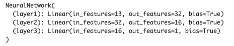
Convert data into a Tensor
In PyTorch, we have to explicitly convert the NumPy array(or pandas DataFrame) into a tensor. The conversion can be performed by “torch.tensor()”, where the param “type” is for specifying a data type.
It must be noted that the data shape of the prediction data will be (***, 1), whereas the data shape of “Y_train” is (***, ). These differences will cause the problem in calculating the loss in training. Therefore, we should reshape the data shape of “Y_train” before converting it into a tensor.
# Convert into tensor
x = torch.tensor(np.array(X_train), dtype=torch.float)
y = torch.tensor(np.array(Y_train).reshape(-1, 1), dtype=torch.float)
Define an Optimizer
We define an optimizer. PyTorch covers many optimization algorithms. The popular and basic ones are SGD and Adam.
Here, we choose the SGD algorithm as an optimizer.
# import torch.optim as optim
optimizer = optim.SGD(model.parameters(), lr=0.005)
We passed the two arguments “model.parameters()” and “lr=0.005”.
The first one is the parameters of the neural network model. The optimizer updates these parameters in each training cycle.
The second parameter is the learning rate. The learning rate is a parameter that indicates how much the model parameters are updated at once. Basically, gradually updating the parameters will surely lead to the optimum solution. On the other hand, it takes time to learn. Therefore, we need to think about the learning rate and find an appropriate value.
If you would like to use Adam as an optimizer, instead of the above codes, specify as follows.
optimizer = optim.Adam(model.parameters(), lr=0.005)Define Loss function
We define a loss function. PyTorch covers many types of loss functions. Here, we use the mean squared error as a loss function.
# define loss function
loss_function = nn.MSELoss()
Train the Model
Finally, we can train the model !
At each epoch, we performs:
- Initialize the gradient of the model parameters
- Calculate the loss
- Calculate the gradient of the model parameters by backpropagation
- Update the model parameters
We set epochs as 200. Then, we repeat the above 200 times.
The loss would be gradually decreasing. It indicates that the training model is being well done !
# Epoch
epochs = 200

for i in range(epochs):
    # initialize the gradient of model parameters
    optimizer.zero_grad()

    # calculate the loss
    y_val = model(x)
    loss = loss_function(y_val, y)
    # Backpropagation
    loss.backward()
    # Update parameters
    optimizer.step()
    if (i % 5) == 0:
      print('epoch: {},'.format(i) + 'loss: {:.5f}'.format(loss))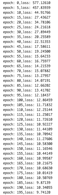
Validation
To validate the performance of the model, we predict the training and validation data. It should be noted here that we have to convert the tensor into the NumPy array after prediction.
# Prediction
Y_train_pred = model(torch.tensor(X_train, dtype=torch.float))
Y_test_pred = model(torch.tensor(X_test, dtype=torch.float))

# Convert into numpy array
Y_train_pred = Y_train_pred.detach().numpy()
Y_test_pred = Y_test_pred.detach().numpy()
Accuracy: R2
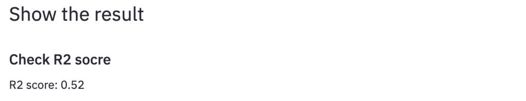
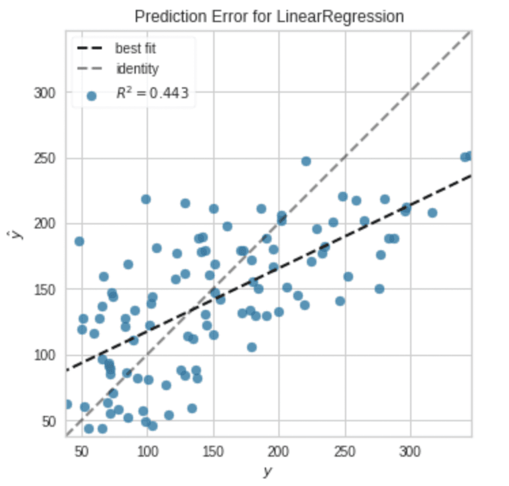
We calculate $R^{2}$ score to confirm the prediction accuracy.
$R^{2}$ is the index for how much the model is fitted to the dataset. When $R^{2}$ is close to $1$, the model accuracy is good. Conversely, when $R^{2}$ approaches $0$, it means that the model accuracy is poor.
We can calculate $R^{2}$ by the “r2_score()” function in scikit-learn.
# from sklearn.metrics import r2_score
R2 = r2_score(Y_test, Y_test_pred)
print(R2)

>> 0.8048130761552106
The score of $0.80$ is better than $0.74$ from linear regression in another post. The accuracy has been improved !
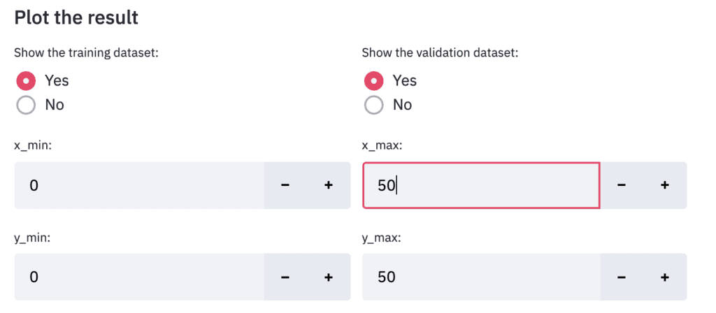
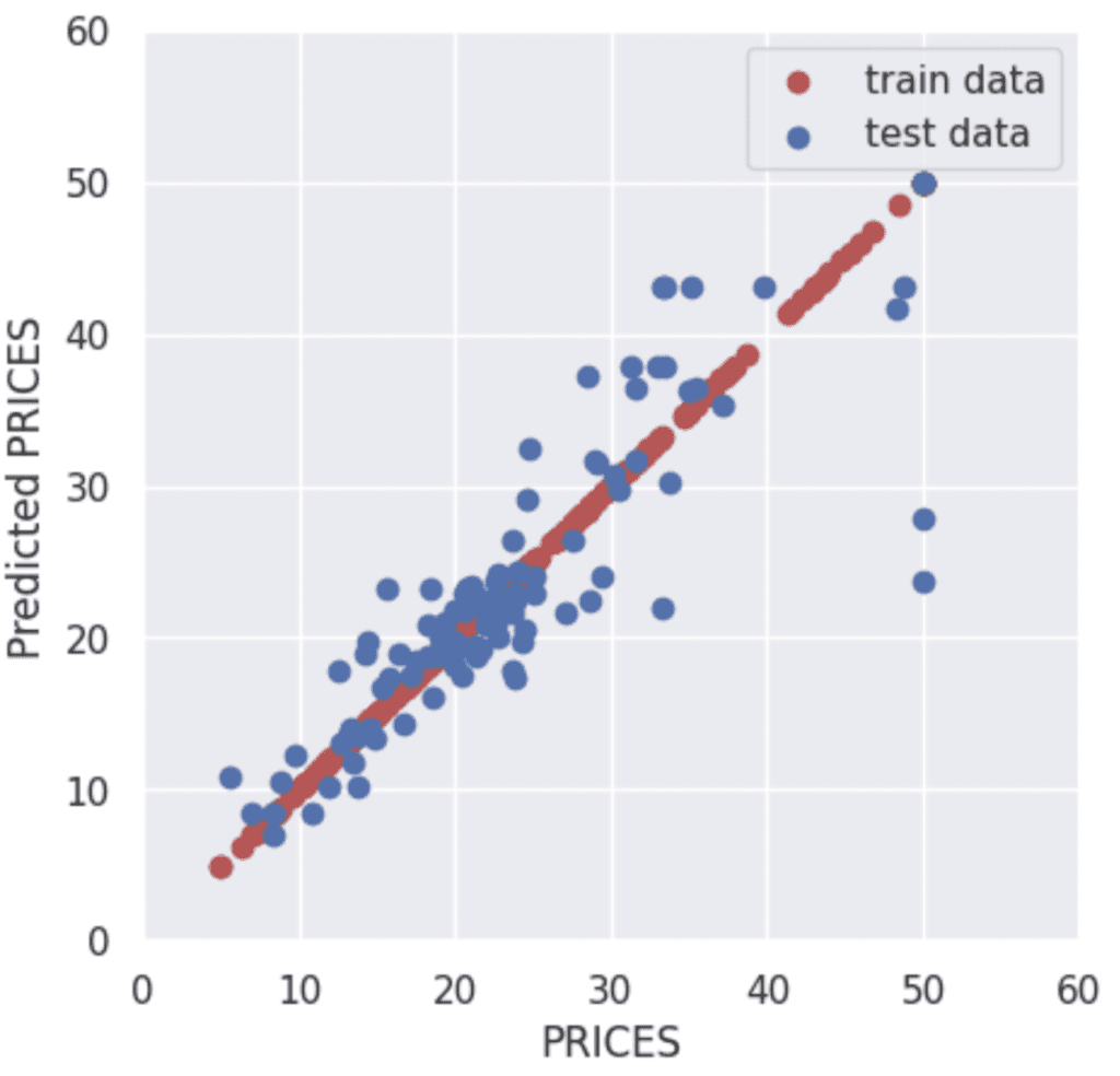
Visualize the Results
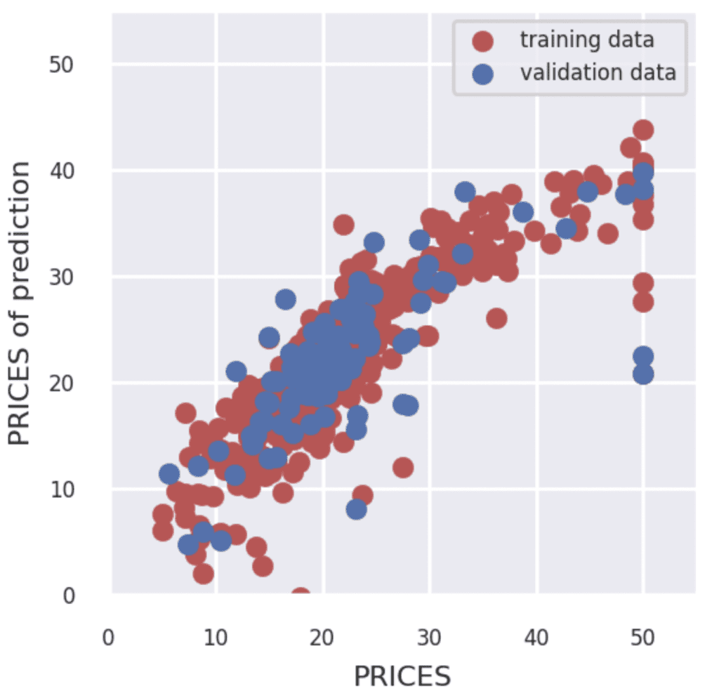
Finally, let’s visualize the results by matplotlib.
The red and blue circles show the results of the training and validation data, respectively.
plt.figure(figsize=(5, 5), dpi=100)
sns.set()
plt.xlabel("PRICES")
plt.ylabel("Predicted PRICES")
plt.xlim(0, 60)
plt.ylim(0, 60)
plt.scatter(Y_train, Y_train_pred, lw=1, color="r", label="train data")
plt.scatter(Y_test, Y_test_pred, lw=1, color="b", label="test data")
plt.legend()
plt.show()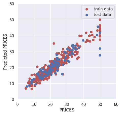
Summary
We have seen the Neural Network analysis constructed by PyTorch against the Boston house prices dataset. Although we use a very simple network structure, the accuracy of the validation data improved more than that of linear regression.
The author hopes this blog helps readers a little.
You may also be interested in:
Step-by-step guide of Linear Regression for Boston House Prices dataset
Step-by-step guide of Decision Tree Regression for Boston House Prices dataset
Brief EDA for Boston House Prices Dataset
Standardization by scikit-learn in Python