Streamlit is a fantastic library, making it easier and faster to make your python script a web app. This library makes it possible to publish your code as a web app! In addition, streamlit is designed with a simple UX, low code, and a readable official document.
In this post, we will see how to set up the environment of streamlit. In another post, we will deploy your data analysis on your web app, i.e., to publish your data analysis code as an interactive format.
Book was published
The new book for a tutorial of Streamlit has been published on Amazon Kindle, which is registered in Kindle Unlimited. Any member can read it !
The execute command is as follows. Your python script(sample.py) will be converted into a web app. A web app will open in a web browser.
$ streamlit run sample.py
Your app can be accessed from a web browser with “localhost:8888” of the URL.
Note that you can kill the web app by “control + C”(for Mac) or “Ctrl + C”(for Windows) in the terminal or the command prompt.
Once you run a python script, you can modify the script interactively. For example, after editing and saving the script, you can confirm the result by reloading the browser.
NOTE) Set up by Docker
If you use docker, it is easy to create an environment for streamlit. You can easily create it from Dockerfile.
FROM python:3.8.8

WORKDIR /opt
RUN pip install --upgrade pip
RUN pip install streamlit==0.78.0

WORKDIR /work
Build a docker image from a Dockerfile. Move the directory where the Dockerfile exists.
$ docker build .
Check the docker image created from Dockerfile by the following command.
$ docker images
Then, create the docker container from the docker image.
$ docker run -it -p 8888:8888 -v ~/(local folder PATH):/(container work directory PATH) <Image ID> bash

# ex.) docker run -it -p 8888:8888 -v ~/streamlit-demo:/work 109bbbac097f bash
You can execute streamlit as follows.
$ streamlit run sample.py --server.port 8888
From the above sequence, your app can be accessed by the URL “localhost:8888” in a web browser.
A set data structure may be unfamiliar to a Python beginner. A set is used for sequence data structures. Therefore, you can have an image against a set like a list, tuple, and dictionary.
First, let’s look at a list as an example. The sample list “sample_list” has six elements, however, whose unique elements are three kinds. The elements are four “apple”, one “orange”, and one “grape”.
You might have encountered the situation that you would like to know the unique elements of a list. Such a situation is the time to use the set() function in Python. Note that the set() is included in Python as a standard module, so you don’t need to import any external module.
It is easy. You just pass the list to the set() function as follows.
Of course, if there are overlaps when we define the elements, these are ignored. Let’s put several “apple” elements in the set when defining. You will see that additional “apple” elements are ignored.
A set is so useful in data science. This is because we have many situations to confirm the overlaps between datasets.
Here is an example. We will check the overlaps of the id column between training and validation datasets. We can do this easily by the set() function and the “intersection” method. The intersection method returns the overlaps elements between two set-type data.
id_train = ["01", "02", "03", "04", "05"]
id_validation = ["04", "05", "06", "07", "08"]

# Into a set data structure
id_train_set = set(id_train)
id_validation_set = set(id_validation)

# Check an overlaps
id_overlap = id_train_set.intersection(id_validation_set)
print(id_overlap)

>>  {'05', '04'}
We have known that the elements of “05” and “04” coexist in the training and validation datasets. From this fact, we should perform a preprocessing, for example dropping overlap data.
Mixing the same information as the training data with the validation data is called data leakage, which leads to an overestimation of accuracy.
Summary
As a sequence data structure, a list, tuple, dictionary are famous. However, a set is practical when we treat unique elements.
You will surely come across a situation where you want to know the unique element of sequence-type data. Recall that there is a set data structure in the Python standard module s at that time.
The famous machine learning algorithms, such as Random Forest and Gradient Boosting Decision Trees(GBDT), are based on the decision tree method. Therefore, it is a good choice to start by learning a decision tree method.
In this post, we will see a brief description of the decision tree method and the sample code. We will apply a regression analysis of the decision tree method to the Boston house prices dataset.
What is a decision tree method?
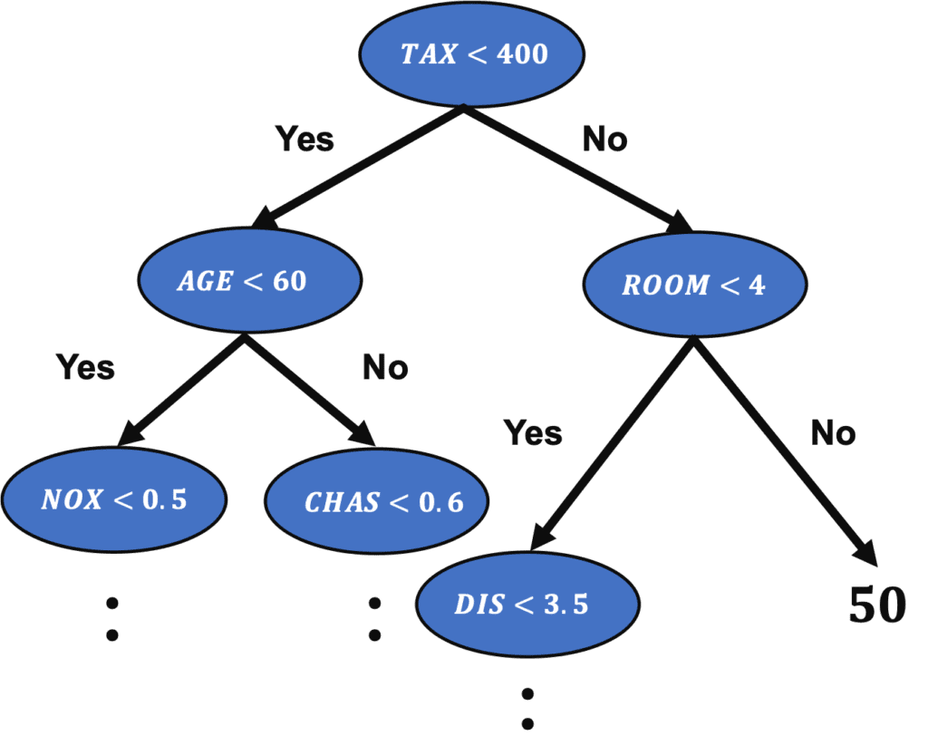
The decision tree is a method of predicting by repeating the case classification of input information. It is recognized as a convenient technique because it can be used for both regression and classification problems.
The model created by a decision tree method becomes more expressive as the number of conditional branches increases. On the other hand, it can be overfitting to the training data, taking into account non-essential conditional branches.
From here, let’s apply a decision tree method to the regression problem.
Load the Dataset
In this post, we use the Boston house prices dataset in the scikit-learn library. We can easily load the dataset by just two lines below.
from sklearn.datasets import load_boston
dataset = load_boston()
The details of the Boston house prices dataset, an exploratory data analysis, is introduced in another post.
import pandas as pd

f = pd.DataFrame(dataset.data)
f.columns = dataset.feature_names
f["PRICES"] = dataset.target
f.head()
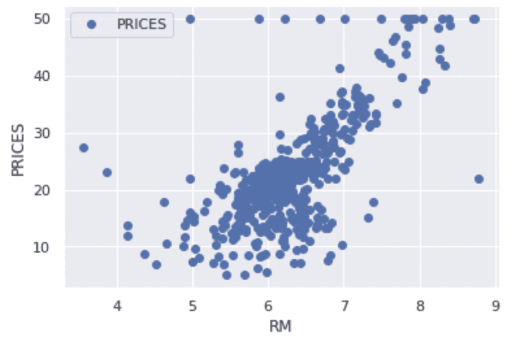
Example: RM vs PRICES
Let’s try to check the correlation between only “PRICES” and “RM”.
import matplotlib.pylab as plt  #-- "Matplotlib" for Plotting

f.plot(x="RM", y="PRICES", style="o")
plt.ylabel("PRICES")
plt.show()
Variables to be used
TargetName = "PRICES"
FeaturesName = [\
              #-- "Crime occurrence rate per unit population by town"
              "CRIM",\
              #-- "Percentage of 25000-squared-feet-area house"
              'ZN',\
              #-- "Percentage of non-retail land area by town"
              'INDUS',\
              #-- "Index for Charlse river: 0 is near, 1 is far"
              'CHAS',\
              #-- "Nitrogen compound concentration"
              'NOX',\
              #-- "Average number of rooms per residence"
              'RM',\
              #-- "Percentage of buildings built before 1940"
              'AGE',\
              #-- 'Weighted distance from five employment centers'
              "DIS",\
              ##-- "Index for easy access to highway"
              'RAD',\
              ##-- "Tax rate per $100,000"
              'TAX',\
              ##-- "Percentage of students and teachers in each town"
              'PTRATIO',\
              ##-- "1000(Bk - 0.63)^2, where Bk is the percentage of Black people"
              'B',\
              ##-- "Percentage of low-class population"
              'LSTAT',\
              ]
We prepare the input and target variables as “X” and “Y”.
X = f[FeaturesName]
Y = f[TargetName]
No need to perform standardization
We don’t need to standardize or normalize the numerical variable in a decision tree analysis. This is because the decision tree classifies the cases by focusing only on the magnitude relationship of the values. Therefore, the difference in the scale of the variables does NOT affect the final result.
Split the Dataset
To validate the performance of the trained model against unseen data, we have to split the dataset into the train data and the test data.
We pass the dataset “(X, Y)” to the “train_test_split()” function. The rate of the train data and the test data is defined by the argument “test_size”. Here, the rate is set to be “8:2”. And, “random_state” is set for reproducibility. You can use any number.
from sklearn.model_selection import train_test_split
X_train, X_test, Y_train, Y_test = train_test_split(X, Y, test_size=0.2, random_state=99)
Create a model instance
We create a decision-tree instance and pass the training dataset to it.
# Fitting Decision Tree Regression to the dataset
from sklearn.tree import DecisionTreeRegressor
regressor = DecisionTreeRegressor()
regressor.fit(X_train, Y_train)
Validation
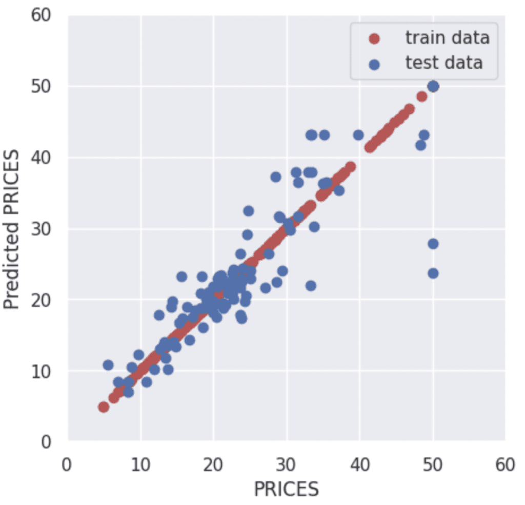
To validate the performance of the model, we predict the training and validation data.
The red and blue circles show the results of the training and validation data, respectively.
To confirm the prediction accuracy of the verification data, we check $R^{2}$ score, the coefficient of determination. $R^{2}$ is the index for how much the model is fitted to the dataset. When $R^{2}$ is close to $1$, the model accuracy is good. Conversely, when $R^{2}$ approaches $0$, it means that the model accuracy is poor.
We can calculate $R^{2}$ by the “r2_score()” function in scikit-learn.
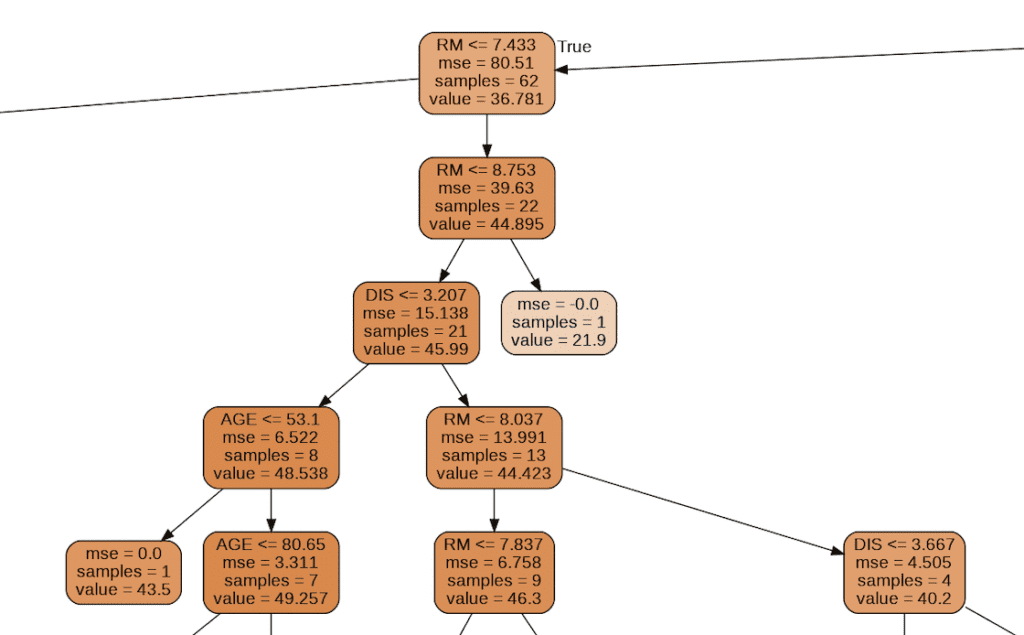
from sklearn.tree import export_graphviz
import pydotplus
from IPython.display import Image
export_graphviz(regressor, out_file="tree-structure.dot", feature_names=X_train.columns, filled=True, rounded=True)
g = pydotplus.graph_from_dot_file(path="tree-structure.dot")
Image(g.create_png())
Summary
We have seen the decision tree analysis against the Boston house prices dataset. In the case of one decision tree model, the accuracy of the validation data is a little worse than the accuracy of the training data. One way to improve accuracy is to use the mean values predicted by multiple models. This is called an ensemble. In the decision tree model base, this ensemble method is called Random Forest and can be easily implemented.
The author hopes this blog helps readers a little.
In this post, we will learn the tutorial of PyCaret from the regression problem; prediction of diabetes progression. PyCaret is so useful especially when you start to tackle a machine learning problem such as regression and classification problems. This is because PyCaret makes it easy to perform preprocessing, comparing models, hyperparameter tuning, and prediction.
Requirement
PyCaret is now highly developed, so you should check the version of the library.
If you have NOT installed PyCaret yet, you can easily install it by the following command on your terminal or command prompt.
$pip install pycaret
Or you can specify the version of PyCaret.
$pip install pycaret==2.2.3
From here, the sample code in this post is supposed to run on Jupyter Notebook.
Import Library
##-- PyCaret
import pycaret
from pycaret.regression import *
##-- Pandas
import pandas as pd
from pandas import Series, DataFrame
##-- Scikit-learn
import sklearn
Load dataset
In this post, we use “the diabetes dataset” from scikit-learn library. This dataset is easy to use because we can load this dataset from the scikit-learn library, NOT from the external file.
We will predict a quantitative measure of diabetes progression one year after baseline. So, the target variable is diabetes progression in “dataset.target“. And, there are ten explanatory variables (age, sex, body mass index, average blood pressure, and six blood serum measurements).
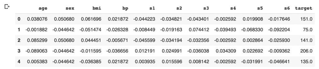
First, load the dataset from “load_diabetes()” as “dataset”. And, for convenience, convert the dataset into the pandas-DataFrame form.
from sklearn.datasets import load_diabetes
dataset = load_diabetes()

df = pd.DataFrame(dataset.data)
It should be noted that we can confirm the description of the dataset.
print(dataset.DESCR)
An excerpt of the explanation of the explanatory variables is as follows.
:Attribute Information:
    - age     age in years
    - sex
    - bmi     body mass index
    - bp      average blood pressure
    - s1      tc, T-Cells (a type of white blood cells)
    - s2      ldl, low-density lipoproteins
    - s3      hdl, high-density lipoproteins
    - s4      tch, thyroid stimulating hormone
    - s5      ltg, lamotrigine
    - s6      glu, blood sugar level
Then, we assign the above names of the columns to the data frame of pandas. And, we create the “target” column, i.s., the prediction target, and assign the supervised values.
Here, we devide the dataset into train- and test- datasets, making it possible to check the ability of the trained model against an unseen data. We split the dataset into train and test datasets, as 8:2.
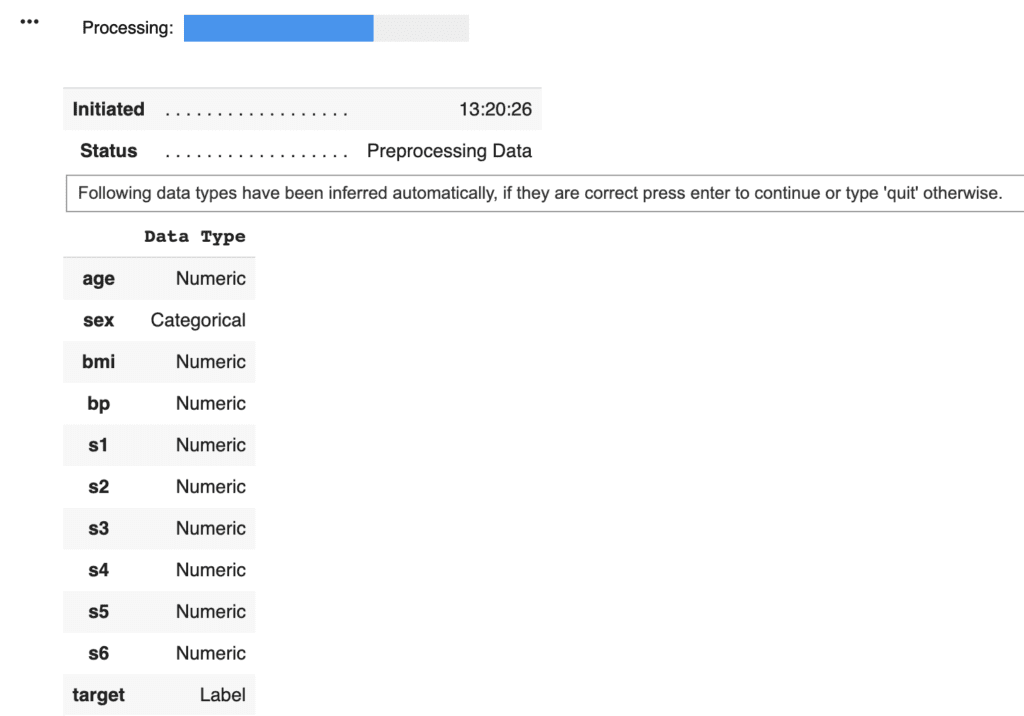
PyCaret needs to initialize an environment by the “setup()” function. Conveniently, PyCaret infers the data type of the variables in the dataset. Due to regression analysis, let’s leave only the numerical data. Namely, we delete the categorical variables. This approach would be practical as a first analysis to understand the dataset.
Arguments of setup() are the dataset as Pandas DataFrame, the target-column name, and the “session_id”. The “session_id” equals a random seed.
model = setup(data = data, target = "target", session_id=99)
PyCaret told us that just “sex” is a categorical variable. Then, we drop its columns and reset up.
data = data.drop('sex', 1) # "1" indicate the columns.
model = setup(data = data, target = "target", session_id=99)
Compare models
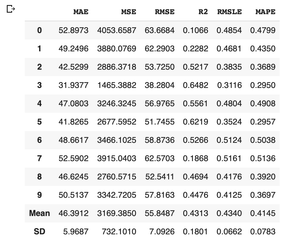
We can easily compare models between different machine-learning methods. It is so practical just to know which is more effective, the regression model or the decision tree model.
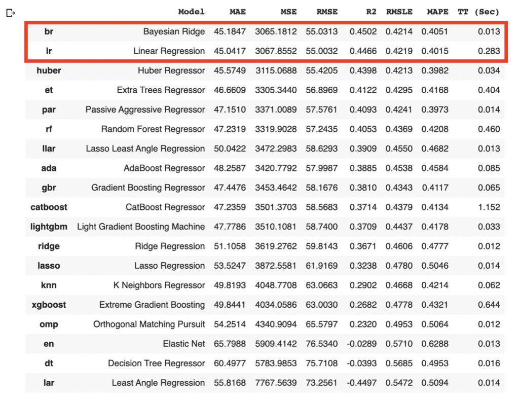
compare_models()
As the above results, the br(Bayesian Ridge) and lr(Linear Regression) have the highest accuracies in the above models. In general, there is a tendency that a decision tree method realizes a higher accuracy than that of a regression method. However, from the viewpoint of model interpretability, the regression method is more effective than the decision tree method, especially when the accuracy is almost the same. Regression analysis tends to be easy to provide insight into the dataset.
Due to the simplicity of the technique and the interpretability of the model, we will adopt lr(Linear Regression) for the models that will be used below. The details of the linear regression technique are described in another post below.
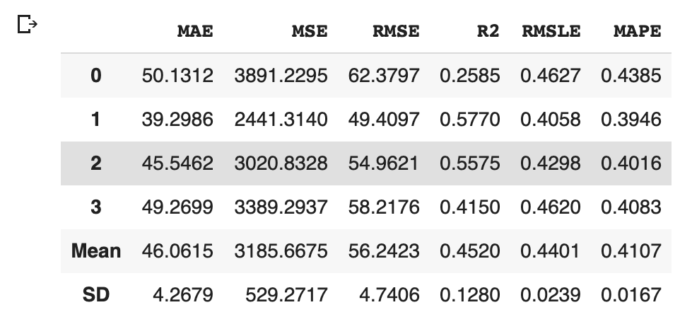
We can create the selected model by create_model() with the argument of “lr”. Another argument of “fold” is the number of cross-validation. “fold = 4” indicates we split the dataset into four and train the model in each dataset separately.
lr = create_model("lr", fold=4)
Optimize Hyperparameters
PyCaret makes it possible to optimize the hyperparameters. Just you pass the object cerated by create_model() to tune_model(). Note that optimization is done by the random grid-search technique.
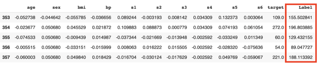
Predict the test data
Let’s predict the test data by the above model. We can do it easily with just one sentence.
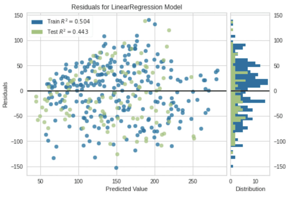
The added column, “Label”, is the predicted values. Besides, we can confirm the famous metric, such as $R^2$.
from pycaret.utils import check_metric
check_metric(predictions["target"], predictions["Label"], 'R2')

>>  0.535
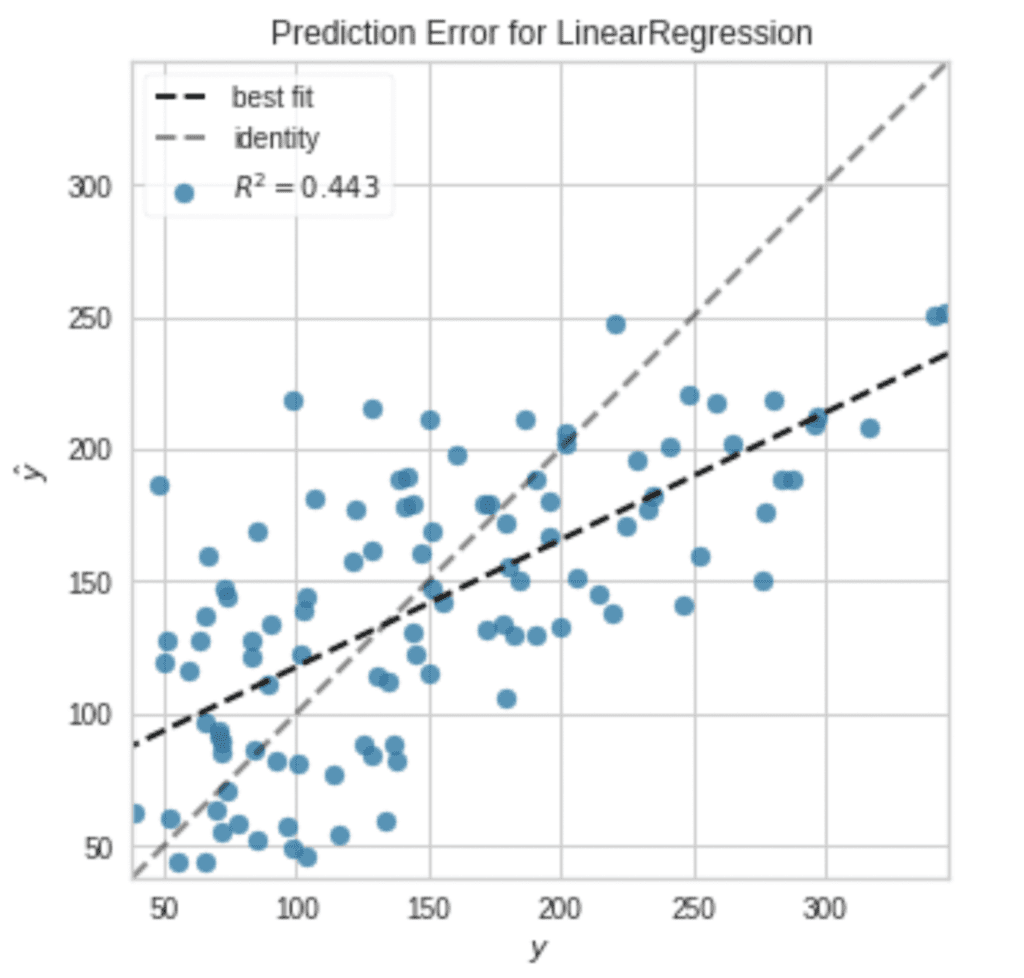
Visualization
It is also easy to visualize the results.
plot_model(tuned_model, plot = 'error')
Note that, without an argument, a residual plot will be visualized.
plot_model(tuned_model)
Summary
We have seen the tutorial of PyCaret from the regression problem. PyCaret is so useful to perform the first analysis against the unknown dataset.
In data science, it is important to try various approaches and to repeat small trials quickly. Therefore, there might be worth using PyCaret to do such thing more efficiently.
The author hopes this blog helps readers a little.
The following contents were already introduced in the previous posts, Part 1 and 2.
variables
comment
arithmetic operations
boolean
comparison operator
list
dictionary
if statement
for loop
function
In this Part 3, we will learn the following contents.
object
class
instance
Note) The sample code in this post is supposed to run on Jupyter Notebook.
object
Python is an object-oriented programming language. An object-oriented style makes it possible to write a more readable and flexible code. Therefore, to understand the concept of an object is highly important.
However, as we have seen in Part 1 and 2, an object-oriented style doesn’t appear. But, it is just Python has hidden object orientation. But from here on, let’s take advantage of object-orientation and take it one step further. This will make your code more functional and maintainable.
Everything that Python deals with is an object. For example, variables, list, function, ..etc. An object is often likened to a thing. In Python, we call a concrete object an instance. The concept of an instance is unfamiliar to beginners. However, please note that it is needed especially when creating a machine learning model.
Example to understand object
Let’s imagine an object with some examples.
First, how about the variable $x$, whose value is $1$.
x = 1
x

>>  1
You may be thinking that $x$ is a variable with the value of $1$. Or, $x$ equals $1$. However, recall the following fact.
type(x)

>>  int
Actually, the variable $x$ has a value of $1$ and the information of data type of “int“. We don’t usually think about the above. However, $x$ is a variable object that has value and data-type information.
We’re not aware of it because we just gave $x$ a value of $1$. But, in behind, Python also gives variable attribute information.
Next, let’s see another example of list.
a = [1, 2, 3]
type(a)

>>  list
The list $a$ has the values of [1, 2, 3] and the information of list. Here, please recall that we can add new element by the append() method.
a.append(10)
a

>>  [1, 2, 3, 10]
When be aware of object, the list object $a$ has the method append() and we called it by $a$.append(). In other words, the append() method was originally included in the list object $a$. The list object has values, information of data type, and functions.
Short summary of object
Could you have imagined an object from the above example? An object is a thing including values, information, and functions. Note that variables, lists, functions, etc. are objects that Python has as standard. We were unknowingly calling and using it.
From here, you will create your own objects with a next topic called “class”. Especially, when creating a machine learning model, we need to create our original object by class(). This is due to designing machine learning models by giving the objects model structure, training, and predictive functions.
class
Here, let’s create our own object by class. The sample code is below. We define a class by “class (class name)”. In the following, we created the class “MyClass()”. And, “__init__()” is for initializing an argument $x$ when we create an instance from the class. Although it is unfamiliar to beginners, a function in class must receive the own argument “self”, which is just an object itself. Then, each function in the class also receives “self”, making it possible to use the variables(self.x) and the functions(func1, func2, func3).
Here, the “__call__()” method is introduced. This method is called without the form of “.method()”. Let’s take the following example. The shaded area is where “__call__()” was added.
Then, create an instance from the class “MyClass_updated()” and call the instance. The point is that the “__call__()” is called at “instance()”.
x = 5
instance = MyClass_updated(x)
instance()  # __call__() is called

>>  25
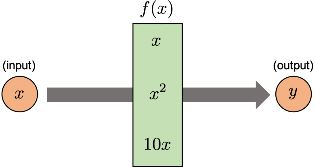
At this point, we can convert $x$, which will vary from $1$ to $10$ in order, with the function $f(x)$. Note that $f(x)$ changes dependent on the range of $x$, whose conditional branching is shown in the figure below.
for x in range(1, 11):
  instance = MyClass_updated(x)
  print( instance() )  # __call__() is called

>>  1
>>  2
>>  3
>>  16
>>  25
>>  36
>>  49
>>  80
>>  90
>>  100
Summary
We have seen an object, class, and instance in Python. These topic may be unfamiliar to beginners. However, these are important especially for a data scientist. The basics of Python are covered in the series of posts of Part 1 – 3.
The next step is to learn the external Python library, such as NumPy, Pandas, and scikit-learn, for data science and machine learning. By calling these libraries from Python, you can take advantage of various functions. For example, NumPy makes it easier to perform numerical calculations. Pandas is useful for the treatment of table data. And, we can create a machine-learning model with low-codes by using scikit-learn.
Note that what you call from an external library is just a class someone created. You have already basic knowledge. And you can also create your own external library.
The author hopes this blog helps readers a little.
A series of posts is intended to see the basics of Python. In the previous post, the following contents were introduced.
Variables
Comment “#”
Arithmetic operations
Boolean
Comparison operator
List
In this post, we will learn the following contents.
dictionary
if statement
for loop
function
instance
class
Note) The sample code in this post is supposed to run on Jupyter Notebook.
dictionary
A dictionary stores pairs of “key” and “value”. We can access the “value” of an element by the “key”.
Here, let’s see the example of a dictionary, which stores fruit names and their numbers. A dictionary is defined by “{ }”. However, when we access the value of the dictionary, we use “[ ]” whose argument is its key.
“if statement” is for a conditional statement, whether True or False. For example, if x is greater than zero, output “x > 0”. On the other hand, if x is less than zero, output “x < 0”. In Python, the above conditional statements are written as follows.
x = 5

if x > 0:
  print( "x > 0" )
elif x < 0:
  print( "x < 0" )
else:
  print( "x = 0")

>>  x > 0
In the above example, when x = 5, x > 0 is True. On the other hand, x < 0 is False. Note that we sometimes forget to add the colon “:”.
How about the input of “x = 0”? You can confirm the output “x = 0”, too.
The if statement branches according to the conditions. Python runs line by line from top to bottom lines.
----------------------------------------------
# condition1, condition2 are True or False.

if condition1:
  Processing 1  # When, condition1 is True
elif condition2:
  Processing 2  # When, condition2 is True
else:
  Processing 3  # When, otherwise
----------------------------------------------
An indent is required at the beginning of the “processing” line. Python recognizes it as processing from whether an indent exists. Note that we sometimes forget to add the colon “:” at the ending of the “if condition”.
It is the same when the variable type is “str”.
x = "orange"

if x == "aplle":
  print( "x is apple." )
else:
  print( "x is NOT apple" )

>>  x is NOT apple
By if statement, we can judge whether the element is included in the list. We use the “in” and “not in” operators.
words = ["orange", "grape", "peach"]

if "apple" in words:
  print( "words includes apple." )
elif "apple" not in words:
  print( "words NOT include apple." )

>>  words NOT include apple.
The point is that the “if(elif)” part is executed when True, and the “else” part is executed when the above does not apply.
Python is an intuitive language so that we can easily confirm the conditions of the above example. From the following example, you can easily understand that if statement branches according to True or False.
"apple" in words  # words = ["orange", "grape", "peach"]
>>  False

"orange" in words  # words = ["orange", "grape", "peach"]
>>  True

x > 0  # x = 5
>>  True
for loop
Repeat the same operation. We use “for loop” in such a case. Here, let’s see the example of printing numbers from 0 to 4.
for i in range(5):
  print(i)

>>  0
>>  1
>>  2
>>  3
>>  4
In the “for loop”, the variable “i” changes in order from 0 to 4.
Note that, in Python, an index starts from 0. And, “range(5)” indicated the five consecutive integers starting from 0. Then, when you would like to print the values from 1 to 5, you should set them as follows.
for i in range(1, 6):
  print(i)

>>  1
>>  2
>>  3
>>  4
>>  5
If you want to skip one, the code is below.
for i in range(1, 6, 2):
  print(i)

>>  1
>>  3
>>  5
It is also possible to output the elements of the list storing the strings in order.
for name in words:  # words = ["orange", "grape", "peach"]
  print(name)

>>  orange
>>  grape
>>  peach
function
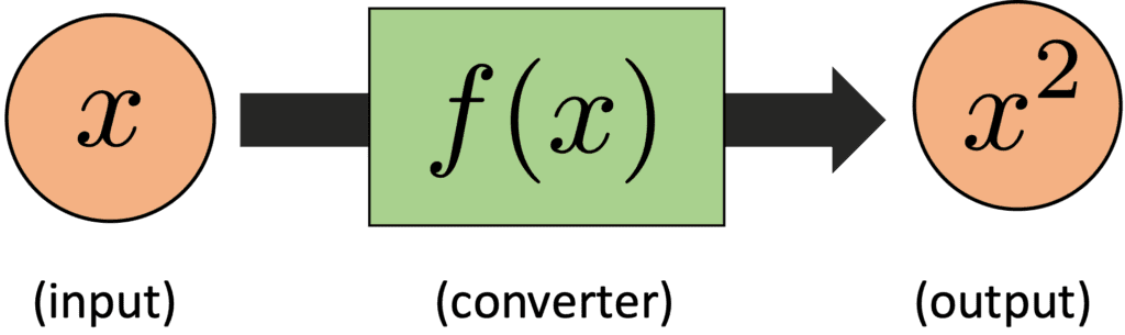
A function is like a converter. For example, we can imagine the typical mathematical function, $f(x) = x^{2}$. The $f(x)$ converts the input $x$ into the output $x^{2}$, whose image is below. And, let’s see the code of this image.
def func(x):
  return x*x

print( func(5) )

>>  25
We defined the function by “def func(x):”, whose name is “func”. And, “x” is an argument, namely an input. And, “return x*x” means this function returns the value of $x^{2}$. Of course, the return value is not always necessary. In the following example, Python just executes the command written in the function “func_print()”.
def func_print():
  print("This is a function")
  print("without a returned value.")

func_print()

>>  This is a function
>>  without a returned value.
Why we use a function? This is because we can understand a code more readable. For example, if we write a set of codes as a function of $f(x)=x^{2}$, we can recognize it as mathematical calculus. In other words, by using a function, the blueprint of your code becomes clearer.
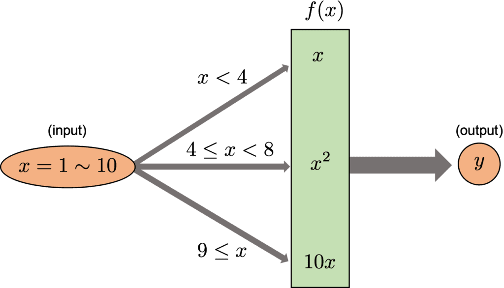
Let’s see the following example for the above description. Here, we consider converting $x$, which will vary from 1 to 10 in order, with the function $f(x)$. Note that $f(x)$ changes dependent on the range of $x$, whose conditional branching is shown in the figure below.
First, we will see the sample code without function.
for x in range(1, 11):
  if x < 4:   # x < 4
    y = x
  elif x < 8: # 4 <= x < 8
    y = x*x
  else:
    y = 10*x  # 9 <= x
  print("x=", x, "was converted into y=", y)

>>  x= 1 was converted into y= 1
>>  x= 2 was converted into y= 2
>>  x= 3 was converted into y= 3
>>  x= 4 was converted into y= 16
>>  x= 5 was converted into y= 25
>>  x= 6 was converted into y= 36
>>  x= 7 was converted into y= 49
>>  x= 8 was converted into y= 80
>>  x= 9 was converted into y= 90
>>  x= 10 was converted into y= 100
Next, the sample code with function is below. We will see that the above code becomes more readable. Especially, it should be easier to understand what is going on in the for loop.
"""
    y = f(x)
"""
def func(x):
  if x < 4:   # x < 4
    return x
  elif x < 8: # 4 <= x < 8
    return x*x
  else:
    return 10*x  # 9 <= x


for x in range(1, 11):
  y = func(x)
  print("x=", x, "was converted into y=", y)

>>  x= 1 was converted into y= 1
>>  x= 2 was converted into y= 2
>>  x= 3 was converted into y= 3
>>  x= 4 was converted into y= 16
>>  x= 5 was converted into y= 25
>>  x= 6 was converted into y= 36
>>  x= 7 was converted into y= 49
>>  x= 8 was converted into y= 80
>>  x= 9 was converted into y= 90
>>  x= 10 was converted into y= 100
In programming, it is very important to write a script with a combination of smaller functional codes. This will make your code easier to read and maintain. In other words, the clearer the blueprint of the code, the better the code.
One more thing you need to know about a function is a local or global variable. A local variable can be accessed just in a function. On the other hand, a global variable can be accessed anytime. Besides, the information of a variable defined in a function is lost after exiting the function.
Let’s understand this explanation through an example. Try to understand how the value of “a” changes with each step.
a = 5
##-- Step 1
print("Step 1: a =", a)
>>  Step 1: a = 5


def func():
  a = 10
  ##-- Step 2
  print("Step 2: a =", a)

func()
>>  Step 2: a = 10


##-- Step 3
print("Step 3: a =", a)
>>  Step 3: a = 5
The above example indicates that the variables of “a” are different between outside and inside of the function “func()”.
Summary
Until here, the core syntax in Python has been introduced. In particular, the main topics (if statement, for loop, and function) are often used, so even beginners of Python should master them.
In the next post, we will try to learn more complex contents.
Python is free and one of the most popular programming languages. You can find that python is simple, flexible, readable, and with rich functions. Python can use external libraries so that we can utilize it in a wide range of fields. Especially, the most popular field is in machine learning and deep learning.
Through some posts, we will see the basics of python from scratch. Let’s take a look at the basic concepts and grammar, keeping in mind the use in data science. Python runs a script line by line. So Python will tell you where you went wrong. So, don’t be afraid to make a mistake. Rather, you can make more and more mistakes and write the code from small stacks with small modifications.
In this post, we will learn the following contents.
Variables
Comment “#”
Arithmetic operations
Boolean
Comparison operator
List
Learning programming is boring as it is basic. However, creative working awaits beyond that !!
Note) The sample code in this post is supposed to run on Jupyter Notebook.
Variables
A variable is like a box for storing information. We assign a name to a variable, such as “x” and “y”. And, we put a value or a string into the variable. Let’s take a glance.
We first put “1” into “x“. And, check the content by the “print()“ function. The “print()” function displays the content on your monitor.
x = 1
print(x)

>>  1
Similarly, strings can also be stored in variables. Strings are represented by ” “.
y = "This is a test."
print(y)

>>  This is a test.
Variables have information of data type, e.g. “int”, “float”, and “str”. “int” is for integer and “float” are for decimal. And, “str” is for a string. Let’s check it by the “type()“ function.
type(x)  # x = 1
type(y)  # y = "This is a test."

>>  int
>>  str

z = 1.5
type(z)

>>  float
Python has the functions to convert variables into “int”, “float”, or “str” types. These functions are “int()”, “float()”, and “str()”.
a = 10

type( int(a) )
>>  int

type( float(a) )
>>  float

type( str(a) )
>>  str
Here, some basic rules for variable name are introduced. It’s okay if you know the following, but see the official Python documentation for more details.
Rules of variable name
It is case sensitive.
Only the alphabet, numbers, and “_” can be used.
The initial letter starts with a number.
For example, “abc” and “ABC” are distinguished. “number_6” is OK, but “number-6” is prohibited. The frequent mistake is including “-“, where “-“ is prohibited. Besides, “5_abc” is also prohibited. The initial letter must be numbers or “_”. However, some variables starting from “_” are for Python itself so that you can’t use them. Therefore, the author highly recommends that variables start from an alphabet, especially for beginners.
Comment “#”
Note that “#” is for comments which are NOT executed by python. Python ignores the contents after “#”. For example as the following one, python regards “print(“Hello world!”)” as a code. The other contents, such as “This is for a tutorial of Python.” and “print the first message!”, are regarded as a comment.
# This is for a tutorial of Python.
print("Hello world!")  # print the first message!
There is another method for comments. Python recognizes as a comment when the statement is between “”” and “””. In the following example, the sentence of “This is a comment.” is skipped by Python.
"""
   This is a comment.
"""
print("test")

>>  test
A comment is so important because we forget what the code we wrote in the past was for. Therefore, programmers leave the explanations and their thought as the comments. Concise and clear. That is very important.
Arithmetic operations
Here, let’s see simple examples of arithmetic operations. Complex calculations are just constructed by simple arithmetic operations. So, most programmers do NOT treat complex mathematics but utilize combinations of simple operations.
Boolean is just True or False. It is, however, important because we construct an algorithm by controlling True or False. For example, we assume the following situation. When an examination score is over 70, it is passed. On the other hand, when the score is less than 70, it is not passed. To control the code by syntax, a boolean is needed.
The concept of a boolean may be unfamiliar to beginners, however, python tells us intuitively. The example below is that the result of judging x > 0(or x < 0) is assigned to the variable “boolean”.
x = 1   # Assign 1 to the variable "x"

boolean = x > 0
print(boolean)

>>  True

boolean = x < 0
print(boolean)

>>  False
There is no problem with the above code. However, the author recommends the following style due to readability. In the following style, we can clearly understand what is assigned to the variable “boolean“.
boolean = (x > 0)
Comparison operator
Here, let me Introduce comparison operators related to Boolean. We have already seen examples such as “<” and “>”. The typical ones we use frequently are listed below.
List is for a data structure, which has a sequence of data. For example, 1, 2, 3,.., we can treat as a group by a list. The list is represented by “[]”, and let’s see the example.
A = [1,  2,  3]
print(A)

>>  [1, 2, 3]
“A” is the list, which stores the array of 1, 2, and 3. Each element can be appointed by the index, e.g. A[0]. Note that, in Python, an index starts from 0.
A[0]

>>  1
It is easy to replace, add or delete any elements. This property is called “mutable”.
Let’s replace the 2 in A[1] with 9. You will see that A[1]will be rewritten from 2 to 9.
A[1] = 5  # A = [1,  2,  3]
print(A)

>>  [1, 5, 3]
We can easily add a new element to the end of the list by the “.append()” method. Let’s add 99 to the list “A”.
Of course, it is easy to delete an element. We do it by the “del” keyword. Let’s delete element 3 in A[2]. We will see that the list “A” will change from “[1, 5, 3, 99]” to “[1, 5, 99]”.
del A[2]  # A = [1,  5,  3,  99]
print(A)

>>  [1, 5, 99]
One more point, the list can handle numerical variables and strings together. Let’s add the string “apple” to the list “A”.
A.append("apple")
print(A)

>>  [1, 5, 99, 'apple']
Actually, this is the thing, where python is different from other famous programming languages such as C(C++) and Fortran. If you know such languages, please imagine that you first declare a variable name and its type. Namely, an array(“list” in Python) can treat only a sequence of data whose variable type is the same.
This is one of the reasons that Python is said to be a flexible language. Of course, there are some disadvantages. One is that the processing speed is slower. Therefore, when performing only numerical operations, you should use a so-called NumPy array, which handles only arrays composed of the same type of variables. NumPy is introduced in another post.
We can easily get the length of a list by the “len()” function.
len(A)  # A = [1, 5, 99, 'apple']

>>  4
Finally, the author would like to introduce one frequent mistake. Let me generate a new list, which is the same for the list A.
B = A  # A = [1, 5, 99, 'apple']
print(B)

>>  [1, 5, 99, 'apple']
B has the same elements as A. Next, let’s replace the one element of B.
We have confirmed that the element of B[3] is replaced from “apple” to “orange”. Then, let’s check A too.
A

>>  [1, 5, 99, 'orange']
Surprisingly, A is also changed! Actually, B was generated by “B = A” so that B refers to the same domain of memory as A. We can avoid the above mistake with the code below.
A = [1, 5, 99, 'apple']
##-- Generate the list "B"
B = A.copy()
B[3] = "orange"  # B[3] = "apple"

print(A) # Check the original list "A"

>>  [1, 5, 99, 'apple']
We have confirmed that the list A was NOT changed. When we copy the list, we have to use the “.copy()” method.
Summary
We have seen the basics of Python with the sample codes. The author would be glad if the reader feels Python is so flexible and intuitive. Python must be a good choice for beginners.
In the next post, we will see the other contents for learning the basics of Python.
Git, a version control system, is one of the essential skills for programmers and software engineers. Especially, GitHub, a version control service based on Git, is becoming the standard skill for such engineers.
GitHub is a famous service to control the version of a software development project. At GitHub, you can host your repository as a web page and keep your codes there. Besides, GitHub has many rich functions and makes it easier to manage the version of codes, so it is so practical for a large-scale project management. However, on the other hand, personal use is a little higher for beginners because of its peculiarity concepts, such as “commit” and “push”.
In this post, we will see the basic usage of GitHub, especially the process of creating a new repository and pushing your codes. It is intended for beginners. And after reading this post, you will keep your codes at GitHub, making your work more efficient.
What is GitHub?
Git, a core system for GitHub, is an open-source tool to control the version of a system. Especially, the function of tracking changes among versions is so useful, making it easier to run a software development project as a team.
GitHub is a well-known service using Git. Roughly speaking, GitHub is a platform to manage our codes and utilize the codes someone has written. We can manage not only individual codes but also open-source projects. Therefore, many open-source projects in the world are published through GitHub. The Python library you are using may also be published through GitHub.
The basic concept of GitHub is to synchronize the repository, like a directory including your codes, between your PC and the GitHub server. The feature is that we synchronize not only the code but also the change records. This is why GitHub is a powerful tool for developing as a team.
Try Git
First of all, if you have NOT installed Git, you have to install it. Please refer to the Git official site.
When Git is successfully installed, you can see the following message after the execution of the “git” command on the terminal or the command prompt.
git

>>  usage: git [--version] [--help] [-C <path>] [-c <name>=<value>]
>>             [--exec-path[=<path>]] [--html-path] [--man-path] [--info-path]
>>             [-p | --paginate | -P | --no-pager] [--no-replace-objects] [--bare]
>>             [--git-dir=<path>] [--work-tree=<path>] [--namespace=<name>]
>>             <command> [<args>]
>>
>>  These are common Git commands used in various situations:
>>  ...
>>  ...
Git command
Here, we will use the Git command. The basic format is “git @@@”, where “@@@” is each command such as “clone” and “add”. In this article, we will use just 5 commands as follows.
For personal use, these five commands are all you need. Each command wii be explained below.
Create a New Repository
First, you create a new repository for your project. A repository is like a folder of your codes. It is easy to create a new repository on your GitHub account.
1. You visit the GitHub site and log in to your account. If you don’t have your account, please create.
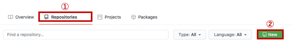
2. Go to the ①“Repositories” tab, and click the ②“New” button.
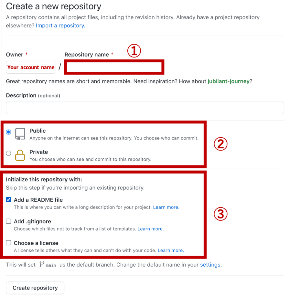
3. Fill in the necessary information, “①Repository name”, “②Public or Private”, and “③Initialized files”.
Note that, in”Public or Private” at ②, “Private” is for paid members. If it’s okay to publish it worldwide like a web page, select “Public”.
Whether you check “Add a README file” depends on you. The “README” file is for the description of your project. Of course, you can manually add the “README” file later.
Clone the Repository
The “clone” command synchronizes the local repository at your PC with the repository at GitHub. You can clone with just only the URL of your repository at GitHub.
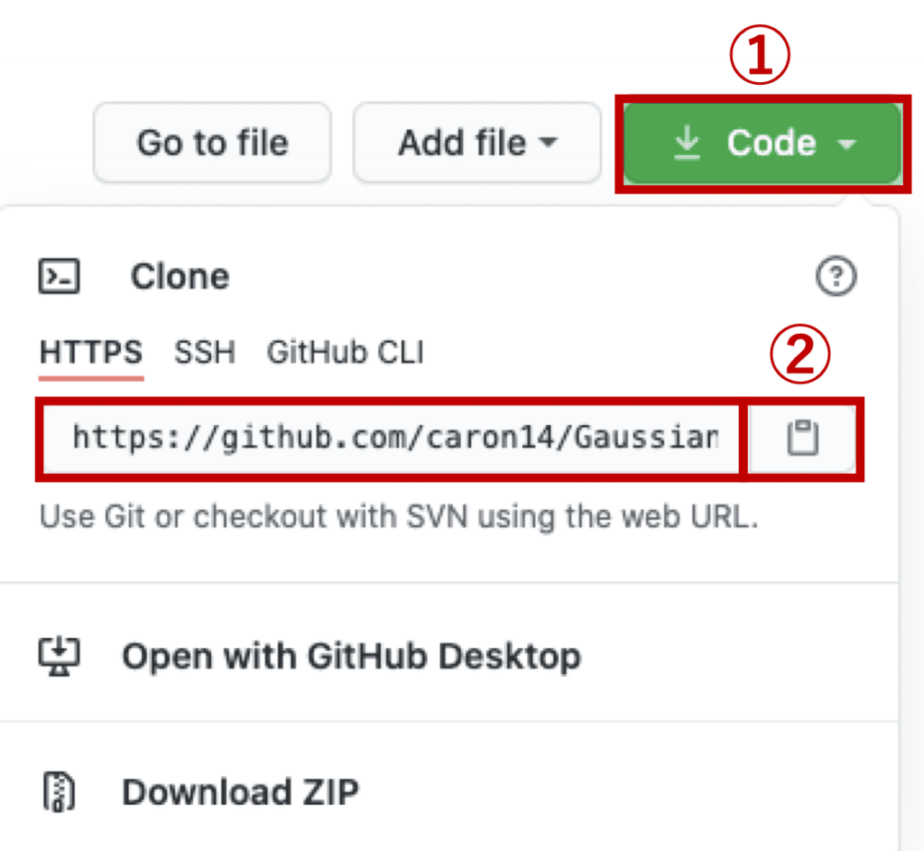
1. Click the green button of “Code”(①).
2. Copy the URL of the HTTPS tab. You can copy by clicking the log at ②. Note that the default setting is for the HTTPS tab.
3. Execute the following command at the working directory on your terminal.
git clone <URL>
When the clone is done successfully, the directory, whose name is the same as the repository name, has been created. The version history of the repository is stored in the “.git” directory. “.git” is the hidden directory, so you can’t see it on your terminal by the “ls” command. You have to use the “ls -a” command. “-a” is the option for hidden files and directories.
Confirm the “Status”
First of all, we have to specify the files to synchronize with the repository on GitHub. Create a new script “sample.py” on the directory you cloned. For example, we can create it with the “touch” command.
touch sample.py
Next, use the “git add” command to put the target file in the staging state. Before executing the “git add” command, let’s confirm the staging condition of the file by the “git status” command.
git status

>>  On branch master
>>  Your branch is up to date with 'origin/master'.
>>
>>  Untracked files:
>>    (use "git add <file>..." to include in what will be committed)
>>
>>  	sample.py
>>
>>  nothing added to commit but untracked files present (use "git add" to track)
“Untracked files:” indicates “sample.py” is a new file. Note that the file is NOT staged yet, so the display of color is with red, “sample.py“. Next, let’s change the status of “sample.py”. We will see the color of “sample.py” will change.
Change the “Status”
We change the status of the file by the “git add” command and check the status again by the “git status” command.
git add sample.py
git status

>>  On branch master
>>  Your branch is up to date with 'origin/master'.
>>
>>  Changes to be committed:
>>    (use "git reset HEAD <file>..." to unstage)
>>
>>  	new file:   sample.py
>>
Git recognized “sample.py” as a new file!
And We have seen the change of color. The display “sample.py” of color has been changed from red to green. The green indicates that the file is now staged!
Note that you can cancel the “git status” command against “sample.py”. After the following command, you will see that “sample.py” was unstaged.
git reset sample.py
Why is the staging need?
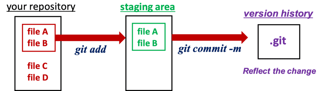
The beginners may be unfamiliar with the concept of “staging”. Why is the staging need? The answer is to prepare for committing. Git reflects the change of a file into the version history when committing. To distinguish the files to commit, Git specifies the files clearly by the “git add” command.
“Commit” the staging files
Next, we will reflect the changes of the staged file to the local repository. This operation is called “commit”. The command is as follows.
git commit -m "This is comment."
“-m” is the option for a comment. The comment makes it possible to understand what is the intention for the change of the code.
The concept of “commit” might be unfamiliar to beginners. Why the commit is need? At the commit stage, Git does NOT reflect the modified files to the GitHub repository but to your local repository. Therefore, when developing as a team, you don’t have to worry about your modification conflicting with your teammate’s modification. At the stage of “push”, your modification of files and the version history are synchronized with the GitHub repository. This is why your teammates can distinguish your changes from those of other people!
“Push” the commited files
The final step is to synchronize your local repository with your GitHub repository. This operation is called “push”. After the “git push” command, the committed changes will be reflected in your GitHub repository.
The command is as follows.
git push
If successfully done, you can confirm on your GitHub web page that your new file “sample.py” exists in your GitHub repository.
Congratulations! This is the main flow of managing files on GitHub.
When you modified the file
From the above, we can see how to add a new file. Here, we have seen the modified file case.
Please add the something change to “sample.py”. Then, execute the “git status” command. You will see Git recognizes the file was modified.
The file is NOT staged yet, so the display of color is with red, “sample.py“.
git status

>>  On branch master
>>  Your branch is up to date with 'origin/master'.
>>
>>  Changes not staged for commit:
>>    (use "git add <file>..." to update what will be committed)
>>    (use "git checkout -- <file>..." to discard changes in working directory)
>>
>>  	modified:   sample.py
>>
The difference is only the above. From here, you do just as you’ve seen.
git add
git commit -m
git push
Summary
We have learned the basic GitHub skill. As a data scientist, GitHub skill is one of the essential skills, in addition to programming skills. GitHub not only makes it easier to manage the version of codes but also gives you opportunities to interact with other programmers.
GitHub has many code sources and knowledge. Why not use GitHub. You can get a chance to utilize the knowledge of great programmers from around the world.
The descriptive statistics have important information because they reflect a summary of a dataset. For example, from descriptive statistics, we can know the scale, variation, minimum and maximum values. If you know the above information, you can have a sense of grasping whether one of the data is large or small, or whether it deviates greatly from the average value.
In this post, we will see the descriptive statistics with a definition. Understanding statistical descriptions not only helps to develop a sense of a dataset but is also useful for understanding the preprocessing of a dataset.
Here, we utilize the Boston house prices dataset for calculating the descriptive statistics, such as mean, variance, and standard deviation. The reason why we adopt this dataset is we can use it so easily with the scikit-learn library.
The code for using the dataset as Pandas DataFrame is as follows.
The details of this dataset are introduced in another post below. In this post, let’s calculate the mean, the variance, the standard deviation for “df[“PRICES”]”, the housing prices.
The mean $\mu$ is the average of the data. It must be one of the most familiar concepts. However, the concept of mean is important because we can obtain the sense of whether one value of data is large or small. Such a feeling is important for a data scientist.
Now, assuming that $N$ data are $x_{1}$, $x_{2}$, …, $x_{n}$, the mean $\mu$ is defined by the following formula. $$\begin{eqnarray*} \mu = \frac{1}{N} \sum^{N}_{i=1} x_{i} , \end{eqnarray*}$$ where $x_{i}$ is the value of $i$-th data.
It may seem a little difficult when expressed in mathematical symbols. However, as you know, we just take a summation of all the data and divide it by the number of data. Once we defined the mean, we can define the variance.
Then, let’s calculate the mean of each column. We can easily calculate by the “mean()” method.
where $N$, $x_{i}$, and $\mu$ are the number of the data, the value of $i$-th data, and the mean of $x$, respectively.
Expressed in words, the variance is the mean of the squared deviations from the mean of the data. It is no exaggeration to say that the information in the data exists in a variance! In other words, there is no worth to pay an attention to the data with the ZERO variance.
For example, let’s consider predicting math skills from exam scores. The exam scores of the person(A, B, and C) are like the below table.
Person
Math
Physics
Chemistry
A
100
90
60
B
60
70
60
C
20
40
60
The exam scores for each subject
From the above table, we can clearly see that those who are good at physics are also good at math. On the other hand, it is impossible to infer whether the person is good at mathematics from chemistry scores. Because all three scores equal the average score of 60. Namely, the variance of chemistry is ZERO!! This fact indicates that the scores of chemistry have no information, no worth to pay attention to. We should drop the “Chemistry” columns from the dataset when analyzing! This is one of the data preprocessing.
Then, let’s calculate the mean of each column of the Boston house prices dataset. We can easily calculate by the “var()” method.
where $N$, $x_{i}$, and $\mu$ are the number of the data, the value of $i$-th data, and the mean of $x$, respectively.
Why we introduced the standard deviation instead of the variance? This is because the unit becomes the same when we adopt the standard deviation of $\sigma$. Then, we can recognize $\sigma$ as the variation from the mean.
Then, let’s calculate the standard deviation of each column of the Boston house prices dataset. We can easily calculate by the “std()” method.
In fact, at the stage of defining these three concepts, we can define the Gaussian distribution. However, I’ll introduce the Gaussian distribution in another post.
Other descriptive statistics are calculated in the same way, so carefully select the ones you use most often and list them below.
Method
Description
mean
Average value
var
Variance value
std
Standard deviation value
min
Minimum value
max
Maximum value
median
Median value, the value at the center of the data
sum
Total value
Confirm all at once
Pandas has the useful function “describe()”, which describes the basic descriptive statistics. The “describe()” method is very convenient to use as a starting point.
“count”: Number of the data for each columns “25%”: Value at the 25% position of the data “50%”: Value at the 50% position of the data, equaling to “Median” “75%”: Value at the 25% position of the data
Summary
We have seen the brief explanation of the basic descriptive statistics and how to calculate them. Understanding the concept of descriptive statistics is essential to understand the dataset. You should note the fact in your memory that the information of the dataset is included in the descriptive statistics.
The author hopes this blog helps readers a little.
Linear regression is one of the basic techniques for machine learning analyses. You may know, in general, other methods are often superior to linear regression in terms of prediction accuracy. However, linear regression has the advantage that the model is simple and high interpretable.
For a data scientist, to understand a dataset is highly important. Therefore, linear regression plays a powerful role as a first step for the purpose of understanding the dataset first.
In this post, we will see the process of a linear regression analysis against the Boston house prices dataset. The author will explain with the step-by-step guide in mind !!
What is a Linear Regression?
Linear regression is based on the assumption of the linar relationship between a target variable and independent variables. Then, if you can represent your dataset well, you can expect a proportional relationship between the independent and objective variables.
In the mathematical expression, the representation of a linear regression is as follows.
From here, let’s perform a linear regression analysis on the Boston house prices dataset!
Prepare the Dataset
In this analysis, we adopt the Boston house prices dataset, one of the famous open datasets published by the StatLib library which is maintained at Carnegie Mellon University. This is because we can use this dataset so easily. Just load from the scikit-learn library without downloading the file.
from sklearn.datasets import load_boston
dataset = load_boston()
The details of the Boston house prices dataset is introduced in another post. But, you can understand the following analysis without referring.
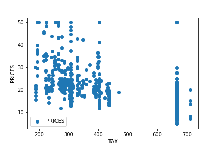
Let’s try to check the correlation between only “PRICES” and “TAX”.
import matplotlib.pylab as plt  #-- "Matplotlib" for Plotting

f.plot(x="TAX", y="PRICES", style="o")
plt.ylabel("PRICES")
plt.show()
At first glance, there seems to be no simple proportional relationship. Including other variables, the EDA(Exploratory data analysis) for this dataset is introduced in another post.
Explicitly define the variables to use for getting from the data frame.
TargetName = "PRICES"
FeaturesName = [\
              #-- "Crime occurrence rate per unit population by town"
              "CRIM",\
              #-- "Percentage of 25000-squared-feet-area house"
              'ZN',\
              #-- "Percentage of non-retail land area by town"
              'INDUS',\
              #-- "Index for Charlse river: 0 is near, 1 is far"
              'CHAS',\
              #-- "Nitrogen compound concentration"
              'NOX',\
              #-- "Average number of rooms per residence"
              'RM',\
              #-- "Percentage of buildings built before 1940"
              'AGE',\
              #-- 'Weighted distance from five employment centers'
              "DIS",\
              ##-- "Index for easy access to highway"
              'RAD',\
              ##-- "Tax rate per $100,000"
              'TAX',\
              ##-- "Percentage of students and teachers in each town"
              'PTRATIO',\
              ##-- "1000(Bk - 0.63)^2, where Bk is the percentage of Black people"
              'B',\
              ##-- "Percentage of low-class population"
              'LSTAT',\
              ]
Get from the data frame into “X” and “Y”.
X = f[FeaturesName]
Y = f[TargetName]
Standardize the Variables
For numerical variables, we should standardize because the scales of variables are different.
In mathematically, the definition of the conversion of standardization is as follows.
Regarding standardization, the details are explained in another post. The standardization is an important preprocessing for numerical variables. If you don’t know standardization, the author recommends that you check the details once.
Here, we split the dataset into the train data and the test data. Why we have to split? This is because we must evaluate the generalization performance of the model against unknown data.
You can see that the above idea is valid because our purpose is to predict new data.
Then, let’s split the dataset. Of course, it is easy with scikit-learn!
from sklearn.model_selection import train_test_split
X_train, X_test, Y_train, Y_test = train_test_split(X_std, Y, test_size=0.2, random_state=99)
We pass the dataset “(X_std, Y)” to the “train_test_split()” function. The rate of the train data and the test data is defined by the argument “test_size”. Here, the rate is set to be “8:2”. And, “random_state” are set for reproducibility. You can use any number. The author often uses “99” because “99” is my favorite NFL player’s uniform number!
At this point, data preparation and preprocessing are fully completed! Finally, we can perform the linear regression analysis!
Create an Instance for Linear Regression
Here, let’s create the model for linear regression. We can perform with the just 3 line code. The role of each line is as follows.
1. Import the “LinearRegression()” function from scikit-learn 2. Create the model as an instance “regressor” by “LinearRegression()” 3. Train the model “regressor” with train data “(X_train, Y_train)”
from sklearn.linear_model import LinearRegression
regressor = LinearRegression()
regressor.fit(X_train, Y_train)
Predict the train and test data
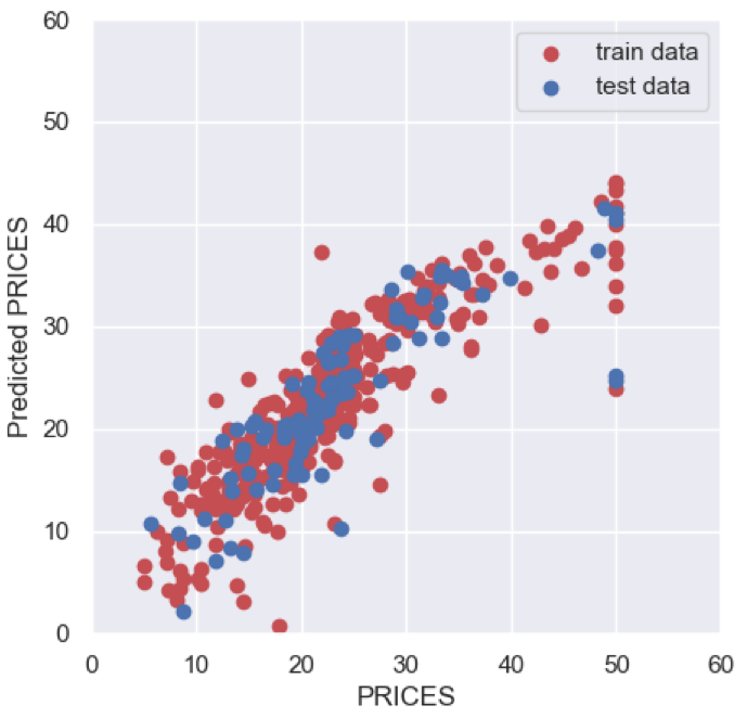
To check the performance of the model, we get the predicted values for the train and test data.
About the above figure, the red and blue circles show the results of the train and test data, respectively. We can see that the prediction accuracy decreases as the price increases.
Here, we check $R^{2}$ score, the coefficient of determination. $R^{2}$ is the index for how much the model is fitted to the dataset. When $R^{2}$ is close to $1$, the model accuracy is good. Conversely, when $R^{2}$ approaches $0$, it means that the model accuracy is poor.
We can calculate $R^{2}$ by the “r2_score()” function in scikit-learn.
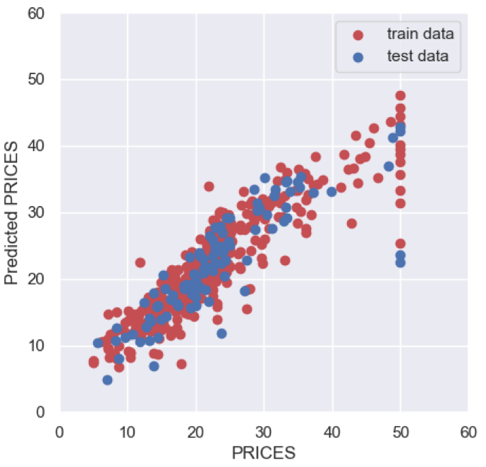
Here, one easy way to improve your score is introduced. The answer is to convert the target variable “PRICES” to a logarithmic scale. Converting to a logarithmic scale reduces the effect of errors in the high “PRICES” range. Reducing the effect of errors between the train data and the predicted values leads to improved models. Logarithmic conversion techniques are often simple and effective and should be helpful to remember.
Then, let’s try!
First, converting the target variable “PRICES” to a logarithmic scale.
Plot the result again as follows. Note that the predicted value is the value after logarithmic conversion, so it must be inversely converted by “np.ep()” when plotting.
We have seen how to perform the linear regression analysis against the Boston house prices dataset. The basic approach to regression analysis is as described here. So, we can apply this approach to other datasets.
Note that the important thing is to have a good understanding of the dataset, making it possible to perform an analysis reflecting the essence.
Certainly, there are several methods that can be expected to be more accurate, such as random forest and neural net. However, linear regression analysis can be a good first step to understanding datasets deeper.
The author hopes this blog helps readers a little.