

Linear regression is one of the basic techniques for machine learning analyses. You may know, in general, other methods are often superior to linear regression in terms of prediction accuracy. However, linear regression has the advantage that the model is simple and high interpretable.
For a data scientist, to understand a dataset is highly important. Therefore, linear regression plays a powerful role as a first step for the purpose of understanding the dataset first.
In this post, we will see the process of a linear regression analysis against the Boston house prices dataset. The author will explain with the step-by-step guide in mind !!
What is a Linear Regression?
Linear regression is based on the assumption of the linar relationship between a target variable and independent variables. Then, if you can represent your dataset well, you can expect a proportional relationship between the independent and objective variables.
In the mathematical expression, the representation of a linear regression is as follows.
$$y =\omega_{0}+\omega_{1}x_{1}+\omega_{2}x_{2}+…+\omega_{N}x_{N},$$
where $y$, $x_{i}$, and $\omega_{i}$ are a target variable, an independent variable, and a coefficient, respectively.
The details of the theory are explained in another post below.
Also, for reference, another post provides an example of linear regression with short code.
From here, let’s perform a linear regression analysis on the Boston house prices dataset!
Prepare the Dataset
In this analysis, we adopt the Boston house prices dataset, one of the famous open datasets published by the StatLib library which is maintained at Carnegie Mellon University. This is because we can use this dataset so easily. Just load from the scikit-learn library without downloading the file.
from sklearn.datasets import load_boston
dataset = load_boston()
The details of the Boston house prices dataset is introduced in another post. But, you can understand the following analysis without referring.
Confirm the Dataset as Pandas DataFrame
Here, we get 3 types of data from “dataset”, described below, as the Pandas DataFrame.
dataset.data: values of the explanatory variables
dataset.target: values of the target variable (house prices)
dataset.feature_names: the column names
import pandas as pd

f = pd.DataFrame(dataset.data)
f.columns = dataset.feature_names
f["PRICES"] = dataset.target
f.head()

>>       CRIM   ZN  INDUS  CHAS  NOX   RM   AGE	 DIS  RAD	TAX PTRATIO	  B   LSTAT PRICES
>>  0   0.00632 18.0  2.31  0.0 0.538 6.575 65.2  4.0900  1.0 296.0 15.3  396.90  4.98  24.0
>>  1	0.02731	 0.0  7.07  0.0 0.469 6.421 78.9  4.9671  2.0 242.0 17.8  396.90  9.14  21.6
>>  2	0.02729	 0.0  7.07  0.0 0.469 7.185 61.1  4.9671  2.0 242.0 17.8  392.83  4.03  34.7
>>  3	0.03237	 0.0  2.18  0.0 0.458 6.998 45.8  6.0622  3.0 222.0 18.7  394.63  2.94  33.4
>>  4	0.06905	 0.0  2.18  0.0 0.458 7.147 54.2  6.0622  3.0 222.0 18.7  396.90  5.33  36.2
Let’s try to check the correlation between only “PRICES” and “TAX”.
import matplotlib.pylab as plt  #-- "Matplotlib" for Plotting

f.plot(x="TAX", y="PRICES", style="o")
plt.ylabel("PRICES")
plt.show()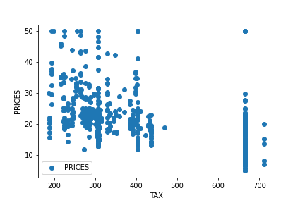
At first glance, there seems to be no simple proportional relationship. Including other variables, the EDA(Exploratory data analysis) for this dataset is introduced in another post.
Pick up the Variables we use
Explicitly define the variables to use for getting from the data frame.
TargetName = "PRICES"
FeaturesName = [\
              #-- "Crime occurrence rate per unit population by town"
              "CRIM",\
              #-- "Percentage of 25000-squared-feet-area house"
              'ZN',\
              #-- "Percentage of non-retail land area by town"
              'INDUS',\
              #-- "Index for Charlse river: 0 is near, 1 is far"
              'CHAS',\
              #-- "Nitrogen compound concentration"
              'NOX',\
              #-- "Average number of rooms per residence"
              'RM',\
              #-- "Percentage of buildings built before 1940"
              'AGE',\
              #-- 'Weighted distance from five employment centers'
              "DIS",\
              ##-- "Index for easy access to highway"
              'RAD',\
              ##-- "Tax rate per $100,000"
              'TAX',\
              ##-- "Percentage of students and teachers in each town"
              'PTRATIO',\
              ##-- "1000(Bk - 0.63)^2, where Bk is the percentage of Black people"
              'B',\
              ##-- "Percentage of low-class population"
              'LSTAT',\
              ]
Get from the data frame into “X” and “Y”.
X = f[FeaturesName]
Y = f[TargetName]
Standardize the Variables
For numerical variables, we should standardize because the scales of variables are different.
In mathematically, the definition of the conversion of standardization is as follows.
$$\begin{eqnarray*}
\tilde{x}=
\frac{x-\mu}{\sigma}
,
\end{eqnarray*}$$
where $\mu$ and $\sigma$ are the mean and the standard deviation, respectively.
Execution code by scikit-learn is just 4 line code as follows.
from sklearn import preprocessing
sscaler = preprocessing.StandardScaler()
sscaler.fit(X)
X_std = sscaler.transform(X)
Regarding standardization, the details are explained in another post. The standardization is an important preprocessing for numerical variables. If you don’t know standardization, the author recommends that you check the details once.
Split the Dataset
Here, we split the dataset into the train data and the test data. Why we have to split? This is because we must evaluate the generalization performance of the model against unknown data.
You can see that the above idea is valid because our purpose is to predict new data.
Then, let’s split the dataset. Of course, it is easy with scikit-learn!
from sklearn.model_selection import train_test_split
X_train, X_test, Y_train, Y_test = train_test_split(X_std, Y, test_size=0.2, random_state=99)
We pass the dataset “(X_std, Y)” to the “train_test_split()” function. The rate of the train data and the test data is defined by the argument “test_size”. Here, the rate is set to be “8:2”. And, “random_state” are set for reproducibility. You can use any number. The author often uses “99” because “99” is my favorite NFL player’s uniform number!
At this point, data preparation and preprocessing are fully completed!
Finally, we can perform the linear regression analysis!
Create an Instance for Linear Regression
Here, let’s create the model for linear regression. We can perform with the just 3 line code. The role of each line is as follows.
1. Import the “LinearRegression()” function from scikit-learn
2. Create the model as an instance “regressor” by “LinearRegression()”
3. Train the model “regressor” with train data “(X_train, Y_train)”
from sklearn.linear_model import LinearRegression
regressor = LinearRegression()
regressor.fit(X_train, Y_train)
Predict the train and test data
To check the performance of the model, we get the predicted values for the train and test data.
y_pred_train = regressor.predict(X_train)
y_pred_test = regressor.predict(X_test)
Then, let’s visualize the result by matplotlib.
import seaborn as sns

plt.figure(figsize=(5, 5), dpi=100)
sns.set()
plt.xlabel("PRICES")
plt.ylabel("Predicted PRICES")
plt.xlim(0, 60)
plt.ylim(0, 60)
plt.scatter(Y_train, y_pred_train, lw=1, color="r", label="train data")
plt.scatter(Y_test, y_pred_test, lw=1, color="b", label="test data")
plt.legend()
plt.show()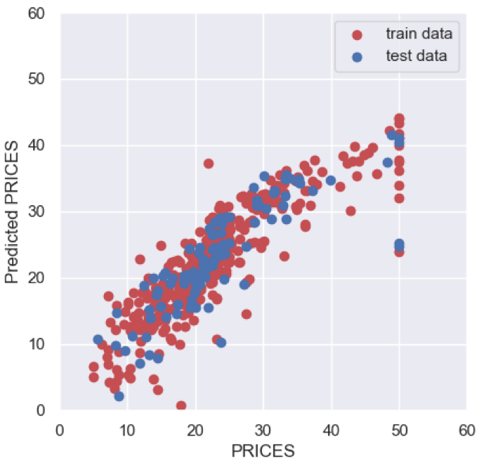
About the above figure, the red and blue circles show the results of the train and test data, respectively. We can see that the prediction accuracy decreases as the price increases.
Here, we check $R^{2}$ score, the coefficient of determination. $R^{2}$ is the index for how much the model is fitted to the dataset. When $R^{2}$ is close to $1$, the model accuracy is good. Conversely, when $R^{2}$ approaches $0$, it means that the model accuracy is poor.
We can calculate $R^{2}$ by the “r2_score()” function in scikit-learn.
from sklearn.metrics import r2_score
R2 = r2_score(Y_test, y_pred_test)
R2

>>  0.6674690355194665
The score $0.67$ is not bad, but also not good.
How to Improve the Score?
Here, one easy way to improve your score is introduced. The answer is to convert the target variable “PRICES” to a logarithmic scale. Converting to a logarithmic scale reduces the effect of errors in the high “PRICES” range. Reducing the effect of errors between the train data and the predicted values leads to improved models. Logarithmic conversion techniques are often simple and effective and should be helpful to remember.
Then, let’s try!
First, converting the target variable “PRICES” to a logarithmic scale.
##-- Logarithmic scaling
Y_log = np.log(Y)
Next, we split the dataset again.
from sklearn.model_selection import train_test_split
X_train, X_test, Y_train, Y_test = train_test_split(X_std, Y_log, test_size=0.2, random_state=99)
And, retrain the model and predict again.
regressor.fit(X_train, Y_train)
y_pred_train = regressor.predict(X_train)
y_pred_test = regressor.predict(X_test)
Plot the result again as follows. Note that the predicted value is the value after logarithmic conversion, so it must be inversely converted by “np.ep()” when plotting.
import numpy as np

plt.figure(figsize=(5, 5), dpi=100)
sns.set()
plt.xlabel("PRICES")
plt.ylabel("Predicted PRICES")
plt.xlim(0, 60)
plt.ylim(0, 60)
plt.scatter(np.exp(Y_train), np.exp(y_pred_train), lw=1, color="r", label="train data")
plt.scatter(np.exp(Y_test), np.exp(y_pred_test), lw=1, color="b", label="test data")
plt.legend()
plt.show()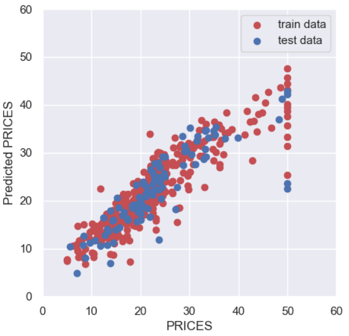
It may be hard to see the improvement from the figure, but when you compare $R^{2}$, you can see that it has improved clearly.
R2 = r2_score(Y_test, y_pred_test)
R2

>>  0.7531747761424288
$R^{2}$ has improved from 0.67 to 0.75!
Summary
We have seen how to perform the linear regression analysis against the Boston house prices dataset. The basic approach to regression analysis is as described here. So, we can apply this approach to other datasets.
Note that the important thing is to have a good understanding of the dataset, making it possible to perform an analysis reflecting the essence.
Certainly, there are several methods that can be expected to be more accurate, such as random forest and neural net. However, linear regression analysis can be a good first step to understanding datasets deeper.
The author hopes this blog helps readers a little.