
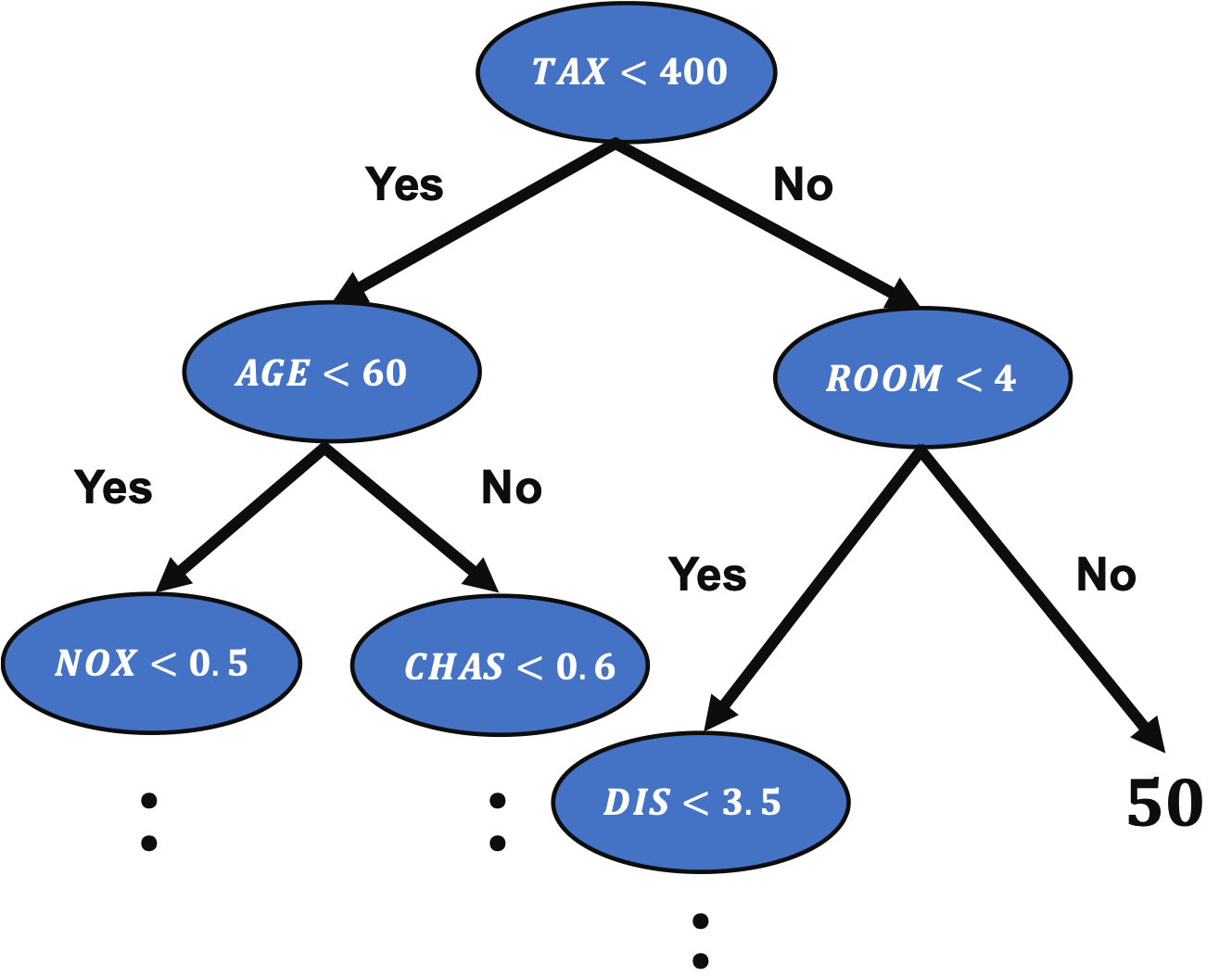
A decision tree method is an important method in machine learning because the famous algorithms, such as Random Forest and Gradient Boosting Decision Trees(GBDT), are based on the decision tree method.
In the previous post, we have seen a regression analysis of the decision tree method to the Boston house prices dataset.
In this post, to improve the accuracy of the model, we will tune the hyperparameters of the model by Grid search.
The full code is in the GitHub repository.
Grid Search
Grid search is a method to explore all possible combinations.
For example, we think about two variables, $x_1$ and $x_2$, where $x_1 = [1, 2, 3]$ and $x_2 = [4, 5, 6]$. In this case, all possible combinations are as follows.
$$[x_1, x_2] = [1, 4], [1, 5], [1, 6], [2, 4], [2, 5], [2, 6], [3, 4], [3, 5], [3, 6]$$
Therefore, computational costs increase proportionally to the number of variables and those levels.
As you can imagine, the disadvantage of grid search is that computational costs increase when the number of variables and those levels become larger.
Baseline of Analysis without tuning the Hyperparameters
First, we import the necessary libraries. And set the random seed.
import numpy as np
import pandas as pd
from sklearn.datasets import load_boston
from sklearn.tree import DecisionTreeRegressor
from sklearn.model_selection import train_test_split
from sklearn.metrics import r2_score
import matplotlib.pylab as plt
import seaborn as sns
sns.set()

random_state = 20211006
In this post, we use the Boston house prices dataset in the scikit-learn library. We can easily load the dataset by just two lines below.
dataset = load_boston()The details of the Boston house prices dataset, an exploratory data analysis, are introduced in another post.
Read the Dataset as Pandas DataFrame
It is convenient to get the data as pandas DataFrame, making it possible to manipulate table data.
# explanatory data
df = pd.DataFrame(dataset.data)
df.columns = dataset.feature_names

# target data
df["PRICES"] = dataset.target

print(df.head())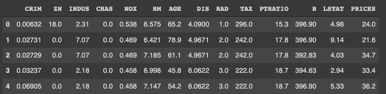
Variables to be used
Here, we prepare the variable-name list. The description of each variable is also described in the comments.
TargetName = "PRICES"
FeaturesName = [
              #-- "Crime occurrence rate per unit population by town"
              "CRIM",
              #-- "Percentage of 25000-squared-feet-area house"
              'ZN',
              #-- "Percentage of non-retail land area by town"
              'INDUS',
              #-- "Index for Charlse river: 0 is near, 1 is far"
              'CHAS',
              #-- "Nitrogen compound concentration"
              'NOX',
              #-- "Average number of rooms per residence"
              'RM',
              #-- "Percentage of buildings built before 1940"
              'AGE',
              #-- 'Weighted distance from five employment centers'
              "DIS",
              ##-- "Index for easy access to highway"
              'RAD',
              ##-- "Tax rate per $100,000"
              'TAX',
              ##-- "Percentage of students and teachers in each town"
              'PTRATIO',
              ##-- "1000(Bk - 0.63)^2, where Bk is the percentage of Black people"
              'B',
              ##-- "Percentage of low-class population"
              'LSTAT',
              ]
We prepare the explanatory and target variables as “X” and “y”.
X = df[FeaturesName]
y = df[TargetName]
No need to perform standardization
We don’t need to standardize or normalize the numerical variable in a decision tree analysis. This is because the decision tree classifies the cases by focusing only on the magnitude relationship of the values. Therefore, the difference in the scale of the variables does NOT affect the final result.
Split the Dataset
To validate the performance of the trained model against unseen data, we have to split the dataset into the train data and the test data.
We pass the dataset “(X, y)” to the “train_test_split()” function. The rate of the train data and the test data is defined by the argument “test_size”. Here, the rate is set to be “8:2”. And, “random_state” is set for reproducibility. You can use any number.
X_train, X_test, y_train, y_test = train_test_split(X, y, test_size=0.2, random_state=random_state)Create a model instance and Train the model
We create a decision tree instance as “regressor”, and pass the training dataset to it.
regressor = DecisionTreeRegressor(random_state=random_state)
regressor.fit(X_train, y_train)
Evaluate the accuracy of the model
To validate the performance of the model, first, we predict the training and validation data.
y_pred_train = regressor.predict(X_train)
y_pred_test = regressor.predict(X_test)
As an indicator of the accuracy of the model, we use the $R^{2}$ score, which is the index for how much the model is fitted to the dataset. The value range is from 0 to 1. When the value is close to $1$, indicating the model accuracy is good. Conversely, when $R^{2}$ approaches $0$, it means that the model accuracy is poor.
We can calculate $R^{2}$ by the “r2_score()” function in scikit-learn.
R2 = r2_score(y_test, y_pred_test)
print("R2 value: {:.2}".format(R2))
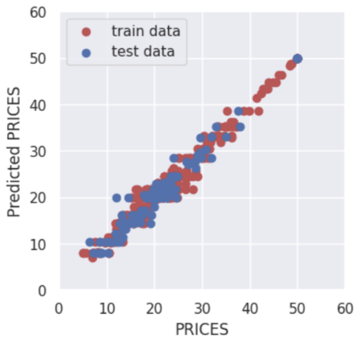
>> R2 value: 0.84The score $0.84$ is not bad.
Besides, visualizing the result is a good choice. The red and blue circles show the results of the training and validation data, respectively.
plt.figure(figsize=(4, 4), dpi=100)
plt.xlabel("PRICES")
plt.ylabel("Predicted PRICES")
plt.xlim(0, 60)
plt.ylim(0, 60)
plt.scatter(y_train, y_pred_train, lw=1, color="r", label="train data")
plt.scatter(y_test, y_pred_test, lw=1, color="b", label="test data")
plt.legend()
plt.show()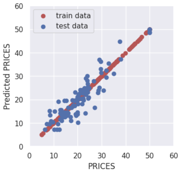
About the above result, what we should pay attention to is the difference of accuracy between train and test data.
Tune the hyperparameters by Grid Search
Then, to improve the accuracy of the model, we tune the hyperparameters of the model by a grid search method.
Before tuning, let’s confirm the hyperparameters of the model.
# Confirm the hyper parameters
print(regressor.get_params)

>>  <bound method BaseEstimator.get_params of DecisionTreeRegressor(ccp_alpha=0.0, criterion='mse', max_depth=None,
>>                        max_features=None, max_leaf_nodes=None,
>>                        min_impurity_decrease=0.0, min_impurity_split=None,
>>                        min_samples_leaf=1, min_samples_split=2,
>>                        min_weight_fraction_leaf=0.0, presort='deprecated',
>>                        random_state=20211006, splitter='best')>
In this post, we tune one of the most parameters, “max_depth”. In the default setting “None”, decision trees can be branched without restrictions. This setting makes it overly easy to adapt to training, i.e., overfitting.
Therefore, we will try to find the optimum solution by setting the number of branches in the range of 1 to 9.
Define the argument name and search range as a dictionary.
# Prepare a hyperparameter candidates
max_depth = np.arange(1, 10)
params = {'max_depth':max_depth}
Next, we define an instance of the grid search, where we pass the decision-tree-model instance and the above dictionary. Note that “cv” and “scoring” indicate the number of folds and metrics for validation, respectively.
from sklearn.model_selection import GridSearchCV

# Define a Grid Search as gs
gs = GridSearchCV(regressor, params, cv=5, scoring='neg_mean_squared_error', return_train_score=True)
Now, we are ready to go. Execute the grid search!
# Execute a grid search
gs.fit(X, y)
After finishing, we confirm the evaluations of the grid search. We check the metrics for each fold.
# Evaluate the score
score_train = gs.cv_results_['mean_train_score']
score_test = gs.cv_results_['mean_test_score']
print(f"train_score: {score_train}")
print(f"test_score: {score_test}")
plt.plot(max_depth, score_train, label="train")
plt.plot(max_depth, score_test, label="test")

plt.title('train_score vs test_score')
plt.xlabel('max_depth')
plt.ylabel('Mean squared error')

plt.legend()
plt.show()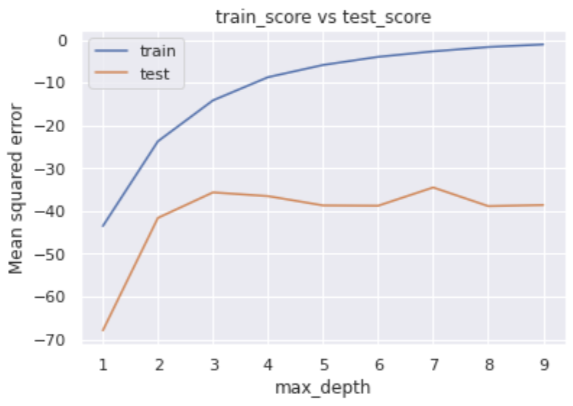
The error for the training data decreases as max_depth increases, while the error for the verification data does not show any significant improvement when the number of branches is 4 or more in the middle.
We can easily check the best parameter, i.e., optimized “max_depth”.
# Best parameters
print(gs.best_params_ )

>>  {'max_depth': 7}
The result suggests that the “max_depth” of 7 is the best.
In addition, we can also get the best model, i.e., when the “max_depth” of 7
# Best-parameter model
regressor_best = gs.best_estimator_
Here, let’s evaluate the $R2$ value again. We will see the model has been improved.
y_pred_train = regressor_best.predict(X_train)
y_pred_test = regressor_best.predict(X_test)

R2 = r2_score(y_test, y_pred_test)
print("R2 value: {:.2}".format(R2))

>>  R2 value: 0.95
It is obvious if you visualize the result.
By adjusting the hyperparameters, the accuracy for the training data is reduced, but the accuracy for the validation data is improved.
In other words, it was a situation of overfitting against the training data, but by setting appropriate hyperparameters, the generalization performance of the model was improved.
Summary
We have seen how to tune the hyperparameters of the decision tree model. In this post, we adopt a Grid Search method. A grid search method is easy to understand and implement.
This time we tried with only one variable, but the case for multi variables can be implemented in the same way. We have defined hyperparameters as a dictionary, but we just need to add additional variables there.
The author hopes this blog helps readers a little.